BME/ME 456 Biomechanics
Calculating Static Muscle Forces using Equilibrium
I. Overview
A significant amount of work in solid and rigid body biomechanics focuses on estimating muscle forces for different tasks. This is for good reason, namely, muscles generate a significant portion of the stresses to which many other tissues are subjected during our daily lives. For some joints like the hip and knee joint, the peak muscle forces may be equivalent to several times body weight. Estimating muscle forces for different anatomic sites however is a very complex task, as demonstrated by the significant amount of ongoing research in this area. The complication comes from the fact that the muscles that generate forces across our joints and tissues are redundant and lead to indeterminant equilibrium system. Still, the use of free body diagrams and static equilibrium remains the starting point for estimating muscle forces. We review the basic concepts of static equilibrium and its application to the musculoskeletal system.
II. Review of Forces and Moments
Forces are represented as vectors in three-dimensional (3D) space, or if we make simplifications in two-dimensional (2D) space. In 3D, the general form of a force vector is:
![]() eq.
1
eq.
1
where F is the total force, Fx is the x component of the force, i is the unit vector along the x axis, Fy is the y component of the force, j is the unit vector along the y axis, Fz is the z component of the force, and k is the unit vector along the z axis.
Moments are defined as the vector cross product between the force vector and the vector between the point which the moment is about the the application of a given force vector:
![]() eq.
2
eq.
2
where x denotes the vector cross product defined as:
![]()
for the ith component of the resulting vector
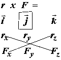
![]()
for the jth component of the resulting vector
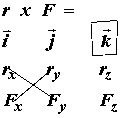
![]()
for the kth component of the resulting vector. The subscripts x,y, and z denote the x,y and z components of the corresponding vector, either the position vector r or the force vector F. Putting it all together, we have the following definition of the vector cross product in 3D for the moment calculation
![]() eq. 3
eq. 3
III. Static Equilibrium Equations (Statically Determinant Systems)
A body is said to be in static equilibrium if the sum if all the forces acting on the body are balanced and all the moments acting on the body are balanced separate from the forces. Balance of forces is termed translational equilibrium since forces will translate the body, while balance of moments is termed rotational equilbrium since moments will rotate the body. The best way to state the required balance of forces and moments is to break down the force balance equations into their x,y and z components. The resulting equations are:
where Fx are the x components of all the forces acting on the body, Fy are the y components of all the forces acting on the body, and Fz are the z components of all the forces acting on the body. We may write the same type of equations for the balance of moments:
As an example of static equilibrium calculation of muscle forces, consider calculating the force required to maintain upper limb position, example 2 in Chapter 1 of the text, as shown below:
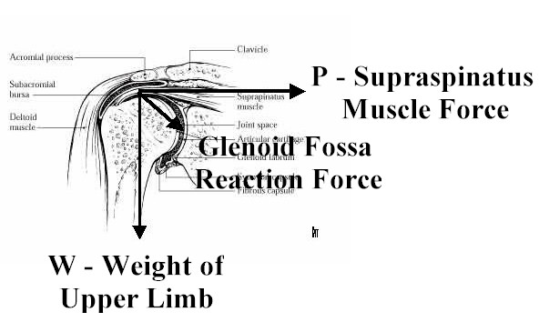
Based on the fact that the position vector r for all forces is zero, there are no moments for the three forces. Thus, the equilibrium equations reduce to translational equilibrium where the sum of the x component of the forces and the y component of the forces is zero. If we assume the angle between the glenoid fossa reaction force and the supraspinatus muscle force is 35 degrees, then we have the following equations:
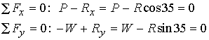
Given that the weight of the upper limb is 50 N, we can calculate the glenoid fossa humerus reaction force as R = W/sin35 = 87.1N. If we plug this result back into the balance of force equation for Fx, we obtain the muscle force necessary to hold the upper limb as 87.1N(cos35) = 71.3N.
The above example did not include moment balance for rotational equilibrium. Consider the following example (Example 3 in Chap. 1 in the text) with the forearm holding a weight (drawn only schematically):
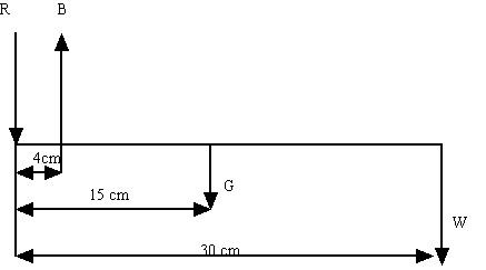
where R is the reaction force at the elbow, B is the muscle force for the biceps, G is the weight of the forearm and W is the weight in the hand. Let W = 20N and G = 15N. In this case, there are no force components in the x direction so we write only force balance in the y direction and a moment balance equation about the elbow. The force balance equation we can write directly as:
![]() eq. 6
eq. 6
For the moment balance about the z axis (coming out of the page), we need to calculate the cross product of the moment arm and the force vector for each applied force. The moment for the reaction force is zero since the moment arm is zero. For the biceps muscle we have the following force vector:
![]()
where the i and k components of the force are zero since the biceps force has only a j component. The moment arm vector is:
![]()
The j and k components are zero since the moment arm is 4 cm only in the x direction. Taking the cross product to obtain the moment we have:
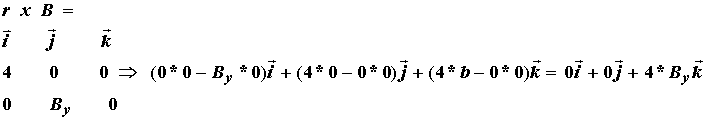
The cross product indicates that we only have a moment in the kth component or z direction. If we follow the same procedure for the other moments, which also only have z components, we obtain the following balance of moments:
![]() eq.
7
eq.
7
Assuming the forearm weight is 15N and the weight in the hand is 20N, we can solve directly for the biceps muscle force magnitude using the moment balance equation (eq. 7):
![]()
Please note that there is a discrepancy in the example in the text. The biceps moment arm is shown as 4cm in Fig.11, but taken to be 3cm in the text and equations. I have used 4cm in my calculations. We can now plug By into the force balance equation (eq.6) to obtain the reaction force as:
![]()
This example illustrates an important concept in biomechanics. Because muscles have short moment arms, they generally must generate large forces to balance external loads.
IV. Static Equilibrium Equations (Statically Indeterminant Problems)
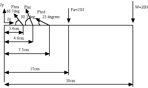
In the above examples we were able to solve for unknown joint reaction and muscle forces using only the static equilibrium equations. However, in most cases of estimating muscle loads, we have redundant muscle forces. This means that there will be more unknowns than equations. Such systems are called statically indeterminate systems. Such a system is illustrated below (this is the example from Fig. 13, page. 17 in the textbook "Basic Orthopaedic Biomechanics"):
where the muscles left to right, their orientation and moment arms are as follows: 1. Biceps brachii (80.3 degrees from horizontal, 4.6 cm from elbow), 2. Brachialis (68.7 degrees from horizontal, 3.4 cm from the elbow) and 3. Brachioradialis (23 degrees from the horizontal, 7.5 cm from the elbow). Let us label the biceps force as Fbic, the brachialis force as Fbra, and the brachioradialis force as Fbrd. Let us assume that these muscles are acting to hold the forearm weight and weight in the hand for the problem we looked at previously. The simplfied Free Body Diagram is as follows:
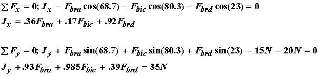
Based on the above free body diagram, we can directly write the balance of force equations for the x and y force components as:
Next, we write the moment balance equation about the z axis. Since the x components of the force do not contribute to the moment (the moment arm is zero), we only have moments generated from the y component of the force. Using the stated moment arms, the moment balance equation is:
What makes this system indeterminate is the fact that we have 5 unknowns (Jx,Jy,Fbra,Fbic,Fbrd) and only 3 equations. This is a statically indeterminate system. This means that there are many possible combinations of values for the muscle forces that will satisfy the equilibrium equation. However, unless we find an alternate approach to solving for muscle force, we cannot find a unique solution.
In biomechanics, there are two widely used approaches to determining a unique solution: 1) Reduction methods and 2) Optimization methods. Reduction methods seek to reduce the number of unknowns to equal the number of equations. Reduction is accomplished using empirical reasoning, experimental data or a combination of the two. For instance, if two muscle groups have similar attachments and perform similar tasks, we may lump their force producing effort together into one muscle group, thus reducing the number of unknown muscle forces by 1. Or we use electromyography (EMG) to measure muscle activation signals, we may be able to deduce that a given muscle is not really active during an activity, again reducing the number of unknowns. The attractiveness of reduction methods is that we can use the same techniques to solve the muscle force problem and that the solution requirements remain relatively simple. This disadvantage is that we may make wrong assumptions, EMG data is often hard to correctly interpret, and we lose detail in terms of muscle prediction.
Reduction Approach Example
As a simple example for the reduction approach, consider the indeterminate system we consider with the forearm holding a weight. Indeterminancy arises because we have 5 unknowns and only three equations. In the reduction method, we would use information that would allow us to eliminate for example two of the three unknown muscle forces. For the first case, let us assume that the biceps and the brachioradialis muscles are not active. Then we have three unknowns (the two components of the joint reaction force and the biceps muscle) and three equations. We can then use the balance of moment equation to solve for the biceps muscle force as:
![]()
The we can use the balance of force in the x direction and y direction to solve for the x and y components of the joint reaction force:
Jx = .17bic = 32.2N ; Jy = .985bic = 186.8N
Likewise, we could assume that the biceps and the brachialis muscles are not active and that only the brachioradialis muscle carries load. We again use the balance of moment equation to solve for the brachioradialis muscle:
![]()
We can then again use the balance of force in the x and y direction to solve for the x and y components of the joint reaction force:
Jx = .92brd = 259N ; Jy = .39brd = 109.8N
Note that depending on what muscles we assume are acitve, we obtain a very different solution even for the joint reaction force. This example shows how sensitive muscle force and joint reaction calculations are to assumptions about muscle activity in the reduction method.
In the second approach, optimization methods, we assume that muscles act together and are recruited in a manner that seeks to mimimize some objective. This has appeal from an evolutionary standpoint in that stronger species survive by using energy efficiently. Optimization techniques in general require numerical solutions. However, over the years they have been shown to be quite powerful in predicting muscle force distributions and are widely used to this day. We next discuss optimization methods and their application to estimating skeletal muscle forces.
 eq. 4
eq. 4 eq.
5
eq.
5