I. Overview

     This is a new class whose purpose is to provide an introduction to Biosolid Mechanics, or more specifically, to provide you with the foundation necessary to study biosolid mechanics, or the mechanics of biological tissues. As such, this class is really divided into two distinct parts:

  1. Introduction to Continuum Mechanics relevant to Biological Tissues
  2. Application of Continuum Mechanics concepts to study Tissue Mechanics

Each section will roughly take half the class. This class itself is really an experiment. Biological tissues are extemely complex, and this holds especially true in their mechanics. In general, biological tissues are nonlinear, visco or poroelastic materials that often undergo large deformations. As such, to cover both hard and soft tissues, it will be necessary to cover some fairly advanced continuum mechanics concepts. In many departments that teach mechanics, the concepts taught in this course are not taught until an advanced undergraduate or even graduate course. These concepts include index notation, finite deformation kinematics, multiple stress definitions, and nonlinear constitutive modeling. Thus, the concepts in this class will be fairly advanced, beyond that of a typical 300 level class. So be forewarned, the mathematics and notation in this class will be advanced. However, without devoting a significant amount of time to continuum mechanics concepts, we would not be able to understand how researchers have studied the mechanics of biological tissues. As such, by the end of the course you should have achieved the following:

    1. Understand and be able to use index notation
    2. Understand the concept of stress and momentum balance
    3. Understand the concepts of small and finite strain
    4. Understand how boundary conditions are determined for biosolid mechanics problems
    5. Understand constitutive models for linear/nonlinear elasticity, viscoelasticity, and poroelasticity
    6. Understand the development of structure-function relationships, that is, how tissue structure relates to defined constitutive models for the following tissues:
         a. musculoskeletal tissues
         b. cardiovascular tissues
         c. pulmonary/abdominal organ tissues
         d. skin, nerve, ocular tissues

II. General Motivation

     The general motivation for this class is to provide you with a general foundation to study Biosolid Mechanics. Of course, one may fairly ask: "Why should I study Biosolid Mechanics? What is it used for?". The applications of biosolid mechanics to clinical medicine are many, although in some ways, these applications are just beginning. For example, clinical applications are as varied as studying how pharmaceuticals used to treat osteoporosis affect bone strength to how diabetes may affect the compliance of arterial walls. Another motivation for studying biosolid mechanics comes from a more basic scientific perspective, namely, many tissues within the body must perform a load bearing function. The question is "How do tissues carry load?". This is a question that many scientists have asked down through the centuries, from Aristotle (384 - 322 BC), who wrote a treatise on the movement of animals,to Galileo Galilee (1564-1642) who surmised that bones gain bending strength by having an increased diameter with hollow center without increasing weight significantly. A interesting concise history of concepts in biosolid mechanics was written by Dr. Bruce Martin and may be found at the website: http://asb-biomech.org/historybiomech/. Thus, biosolid mechanics covers the range from basic to applied science, with significant applications in medicine. In the rest of this overview, I will present some applications of biosolid mechanics to clinical issues including hypertension, osteoporosis, and low back pain. The purpose of these examples is twofold. First, it is to motivate you as to the importance of biosolid mechanics for critical problems in human medicine. Second, it is to motivate you by the complexity of the models to study continuum solid mechanics as a basis understanding biosolid mechanics models.

III. Osteoporosis - a motivation for studying bone mechanics and linear elasticity

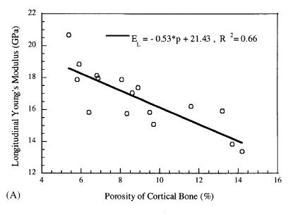
      A basic premise of aging is that we lose bone mass, and with the loss in bone mass our bones become less stiff and have less strength. This premise raises one of the fundamental issues in biosolid mechanics, that of structure-function. Indeed, one of the biggest uses of biosolid mechanics is to relate changes in tissue structure to changes in its function. One important area of research is to determine how bone structure is related to its elastic and failure properties. This has important applications in osteoporosis, both for diagnosing which osteoporotic patients are at risk for fracture, and for evaluating how potential pharmaceutical treatments that alter bone structure can alter bone mechanical behavior. One of the fundamental structural parameters of bone is porosity. Thus, a good starting place is to try and understand how porosity affects not only the overall magnitude of bone properties, but the different ratio of stiffness in different directions. A recent paper in biomechanics by Dong and Guo (2004) reexamined this question in femoral cortical bone. They measured a structural component (porosity) and related this to mechanical measures of bone stiffnes (five anisotropic linear elastic constants, including a transverse and longitudinal Young's modulus, a transverse and longitudinal shear modulus, and Poisson's ratio. The schematic for this study is shown below:

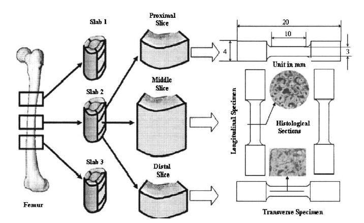
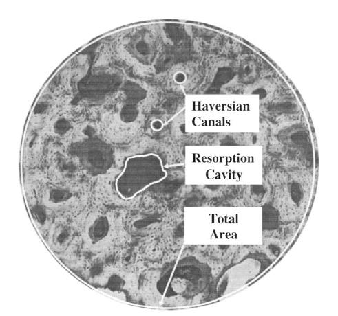
Dong and Guo measured the porosity as a structural measure of bone as below:

Not unexpectedly, Dong and Guo found that the longitudinal Young's modulus decreased with increasing porosity. However, somewhat surpisingly, the transverse moduli did not show a dependence on porosity. The two plots showing these results are below:

          

These results demonstrate the importance of structure-function relationships for tissues. If a drug and stop bone loss, we would expect femoral cortical bone.

Taking this idea one step farther, Cody et al. (1999) used density-modulus relationships in patient specific finite element models to predict failure load. They compared the finite element model, which uses a site specific structure-function relationship of density modulus, to an overall density failure load prediction. The finite element model is shown below:

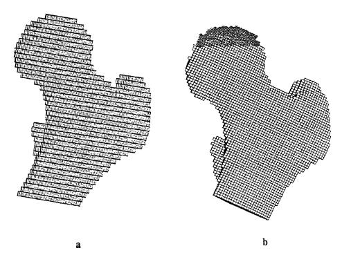
Results demonstrated that the patient specific finite element models incorporating local structure-function relationships did a better job of predicting femoral failure than only density failure relationships. This is shown in the graph below:

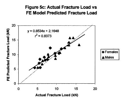
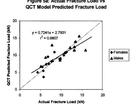
These results demonstrate the promise of bone structure-function relationships in helping to predict bone fracture due to age and osteoporosis.

IV. Hypertension - a motivation for studying blood vessel mechanics and nonlinear elasticity

      Hypertension, or high blood pressure, is a significant health problem worldwide. Hypertension is a risk factor in a number of other health problems, including stroke, heart failure, intracranial hemorrhage, and atherosclersosis (Humphrey, 2002). Although it is widely accepted that there is a link between hypertension and blood, the plethora of data can often be confusiong. For example, it is known that blood vessels become stiffer with age, and that this increased vascular stiffness will lead to increased blood pressure, heart failure, and heart attack (http://www.sciencedaily.com/releases/2001/09/010906072321.htm). Also, a recent study in the American Journal of Hypertension by Grey et al. (2003), noted that increased small artery stiffness was signficantly correlated with a higher occurence of cardiovascular events. Furthermore, Grey et al. found that diet and family history factors including high cholesterol, high blood pressure and diabetes were associated with an increased artery stiffness. It is also known that when hypertension is induced, that this leads to remodeling of blood vessels (that is, a change in blood vessel structure) which in turn leads to a change in blood vessel mechanical properties, generally increasing this properties. Thus, hypertension and blood vessel stiffness may be a postive feedback loop, with one factor increasing the other and vice versa.

     Although measures of pulse velocity are related to arterial compliance, we would like to have a very quantitative measure of arterial stiffness to compare between individuals or disease states. As such, we would like to utilize a nonlinear elasticity constitutive model to characterize changes in blood vessels. We now illustrate the use of such nonlinear constitutive models.

    In a recent paper, Schulze-Bauer and Holzapfel (2003, J. Biomechanics), proposed a method to determine nonlinear constitutive models for human arteries from clinical data using a strain energy function. There method was based on two assumptions:

   1. The axial stretch and axial force of the artery are independent from internal pressure

   2. The ratio of circumferential to axial stress is known for one pressure

The first assumption has been shown for rat, rabbit and dog arteries. The second assumption was taken from rabbit arteries. Then, Schulze-Bauer and Holzapfel proposed a strain energy function of the form:

   

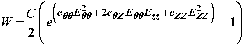
where W is the strain energy function, Eqq and Ezz are components of the finite strain tensor, and C, Cqq, Cqz, and Czz are constants that are to be determined experimentally. By differentiating the strain energy function with respect to the strain components, we can obtain the 2nd Piola-Kirchoff stress components. This can of course be done analytically by hand, but it can also be done using symbolic manipulation software available in MATLAB or MATHEMATICA. The following script shows how this may be done in MATLAB:

First, we define the symbols for the above strain energy function:

>> syms cqq cqz czz c eqq ezz

Note that the subscript "q" denotes q, since q cannot be typed directly in MATLAB. Next, we define the strain energy function in terms of these constants:

>> w = 0.5*c*(exp(cqq*eqq^2 + 2.*cqz*eqq*ezz + czz*ezz^2) - 1)

w =

1/2*c*(exp(cqq*eqq^2+2*cqz*eqq*ezz+czz*ezz^2)-1)

Finally, we can differentiate the strain energy function to obtain the second Piola-Kirchoff stress tensor components. If we first differentiate the strain energy function with respect to eqq, we obtain the stress component sqq as:

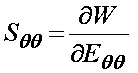
To do this in MATLAB, we simply type:

>> sqq = diff(w,'eqq')

sqq =

1/2*c*(2*cqq*eqq+2*cqz*ezz)*exp(cqq*eqq^2+2*cqz*eqq*ezz+czz*ezz^2)

We obtain the same result as if we had differentiated the strain energy function analytically:

we can do the same procedure to obtain the Szz stress component as:

Again, in MATLAB we type:

>> szz = diff(w,'ezz')

szz =

1/2*c*(2*cqz*eqq+2*czz*ezz)*exp(cqq*eqq^2+2*cqz*eqq*ezz+czz*ezz^2)

or again the same as we could obtain analytically:

The constants to be determined experimentally in a constitutive model reflect the underlying physiologic state of the tissue. As such, we can use constitutive models to construct structure-function relationships for tissues, that can relate the physiology or tissue structure, to its function. Schulze-Bauer and Holzapfel were able to obtain fit the above model to experimentally measured pressure-diameter relationships for a 50 year old patient with normal blood pressure and a 52 year old patient with hypertension. The data was obtained by Stefanadis (1995) using an ultrasonic pressure catheter. By fitting the experimental data, Schulz-Bauer and Holzapfel obtained the following experimental coefficients:

Normal Blood Pressure Patient: C(KPa) =  15.4 ;  cqq =   2.13 ;  cqz =   1.5 ;  czz =  1.1 

Hypertensive Patient:                 C(KPa) =  24.4 ;  cqq =   7.35 ;  cqz =   4.07 ;  czz =  2.44

One immediate question is how well the constitutive model can match experimental results. Schulze-Bauer and Holzapfel compared the experimental pressure versus inner diameter of the artery to that predicted by the constitutive model. The open squares represent the experimental data while the solid line represents the prediction from the constitutive model:

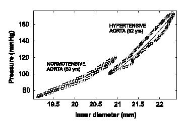
As we can see, the constitutive model matches the experimental data very well, indicating the assumptions made in creating the constitutive model are reasonable. Once the constitutive modeling approach is valid, we can then use it to predict the stress-strain behavior of this artery in both the normal and hypertensive patient. Note, however, that if we wish to predict the mechanical behavior of arteries in other patients, or even different arteries in the same patient, it is highly likely that we will need to measure new coefficients for the constitutive model, although the constitutive model itself may take the same form. Schulze-Bauer and Holzapfel also predicted the stress-strain behavior (in this case, strain is represented as a stretch ratio) for the normal and hypertensive patient and obtained the following:

               

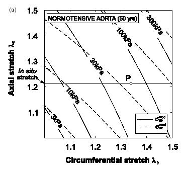
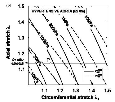
                      Normal Patient                                                                                     Hypertensive Patient

As we can see from the graphs, the artery in the hypertensive patient develops significantly more stress than the artery in the normal patient. Specifically, if we at the data for a stretch of 1.4 in both the axial and circumferential direction, we can see that the patient with the normal artery develops a sqq stress of about 150 KPa, while the artery in the hyptensive patient develops a stress of about 3 MPa, an increase of nearly 20 times

IV. Low Back Pain and Disc Degeneration- a motivation for studying intervertebral disc mechanics and nonlinear elasticity and poroelasticty

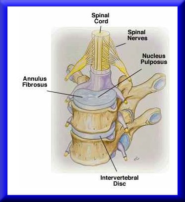
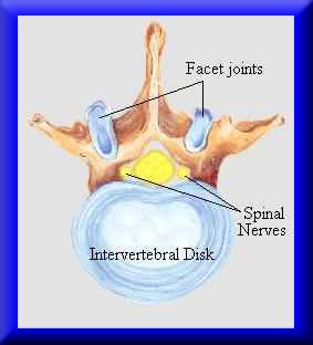
      Intervertebral disk degeneration is a leading cause of low back pain that debiltates many people in the US. In fact, low back pain is the leading cause of disability in people under the age of 45. In addition, between $20 and $50 billion is spent every year for treatment cost and disability payments related to back pain (http://yourmedicalsource.com/library/backpain/BAK_whatis.html). Although a very small percentage of the population with back pain end up requiring surgical treatement, there are still over 300,000 spine fusion operations performed in the US every year. Spine fusions are typically performed subsequent to degenerated disk. Degeneration of spinal discs is hypothesized to result from mechanical insult. Adams et al. (Spine, 2000, 25:1625-1636) showed that mechanical damage in the annulus fibrosus would compound and worsen, leading to reduced pressure in the nucleus pulposus. Pictures of the intervertebral disc from the site: http://www.thespinepage.com/anat.htm, by Drs. William Reed, Jr. and Glenn Amundson:

                

The goal in biosolid mechanics of the intevertbral disc is to develop a constitutive equation that accurately reflects the mechanical behavior of the intervertebral disc. As we will often see is the case with biological tissues, there are different classes of constitutive models that have been developed to describe intervertebral disc behavior. We will briefly touch on examples of two widely used models: nonlinear elasticity and poroelasticity.

A nonlinear anisotropic elastic constitutive model was proposed for intervertebral disk by Klish and Lotz (1999, J. Biomechanics). Since the annulus fibrous contains oriented collagen fibrils. Klisch and Lotz proposed a strain energy function that included terms that accounted for the fibril orientation. Essentially, the collagen fibrils constitute a "net" that helps constrain the fluid filled nucleus pulposus in the center. Klisch and Lotz idealized this fiber net using the following geometric model:

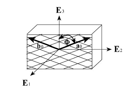
where E1, E2, and E3 are unit vectors in the radial, circumferential, and axial directions respectively. The angle f defines the angle between the two vectors describing the fibril direction with the axial direction. Thus, the vectors a0 and b0 are defined as:

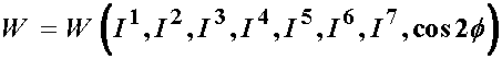
Based on the idea that the fibril orientation will produce a locally orthotropic material, a strain energy function can be in terms of seven invariants:

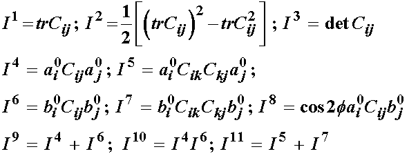
The In quantities in the strain energy function are invariants of the right Cauchy deformation tensor, and are defined as:

The first general model proposed by Klisch and Lotz had a strain energy function of the form:

 

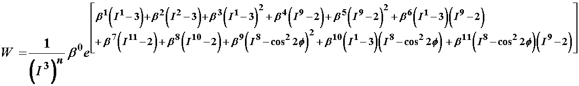
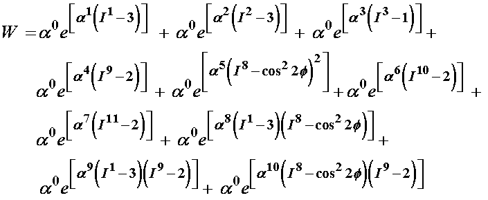
where n and all the b terms are coefficients that must be determined by experiment. Since the above model was very senstive during the curve fitting process, Klisch and Lotz later chose a second strain energy function, given below:

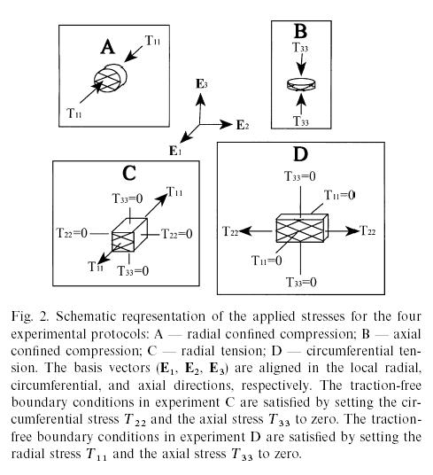
where again the a terms are coefficients to be determined by experiment. To determine the experimental coefficients, Klisch and Lotz fit both strain energy functions to experimental data from Iatridis et al. (1998). Iatridis performed the following mechanical tests of intervertebral body tissue:

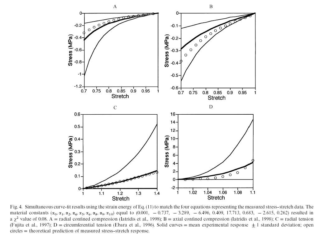
By curve fitting data from the second model, Klisch and Lotz could show good agreement between their constitutive model and experimental data for the normal vertebral body from Iatridis et al. (1998) as shown below, where the circles are the model results and the solid lines represent the mean behavior and +/- 1 standard deviation:

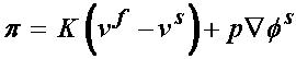
This showed that the nonlinear elastic model could fit the equilibrium behavior of the intervertebral disk. However, in reality, the intervertebral disk, like many biological tissues, is a combination of a solid and fluid. Therefore, load bearing for time dependent loads is in reality shared between the fluid component and the solid compoent. In fact, if the tissue is permeable, then the fluid flows out more easily and there is a quicker transition between solid and fluid load sharing. In fact, in the original article by Iatridis et al. (1998), the intervertebral disk was modeled using poroelasticity, whether is a mechanics theory that accounts for fluid/solid coupled behavior. In this case, constitutive equations are developed for both the fluid and solid phases. The fluid is assumed to be incompressible with the following constitutive equation:

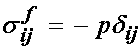
The solid phase stress is:

where the last term represents the elastic stress in the solid component. This was represented by Iatridis using the following constitutive model:

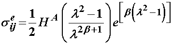
where here, Ha is an equilibrium modulus, the stiffness of the tissue after all the fluid has flowed out, l is a stretch ratio, and b is a constant to be determined experimentally. In addition, there is a drag force that couples the fluid and solid behavior, due to the fluid flowing out of the solid. This is given by:

K is the drag coefficient. This is related to the inverse of the permeability by:

where the small "k" is the permeability. Thus, we see that the smaller the permeability, the higher the drag force between fluid and solid. Finally, the permeability depends on the strain and may be written as:

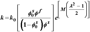
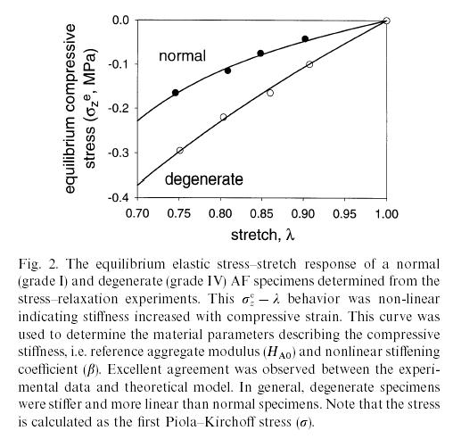
where k0 and M are constants to be fit with experiments from tissues. Iatridis compared the constitutive model coefficients Ha, b, and k0 for normal human cadaver intervertebral disks and degenerated intervertebral disks. Interestingly, they found that the degenerated disks exhibited more linear behavior, (smaller value of b), but were in general stiffer (higher value of Ha). This is reflected in the graph below:

However, Iatridis et al. found no significant difference between the permeability of normal and degenerated disks. Note that both of these results could have been determined with either the Klisch and Lotz constitutive model, or the Iatridis constitutive model. Either way, however, the use of the constitutive model allowed quantification of how a tissues morphological state (normal vs. degenerated) affected its function.

V. Summary

      Understand all this? Any of this? None of this? Don't worry! I don't expect you to understand any of this at this point. That is the purpose of the class! By the end of the class, if you flip back to this section, you should be able to understand all of this! The point of this section is both to motivate you and forewarn you. To motivate you, I have tried to pick examples that show biosolid mechanics has important applications in human health. To forewarn you, I have chosen examples that demonstrate the difficulties of studying biosolid mechanics, namely that it can be very complex. That is why we will spend nearly half the term studying the continuum mechanics basis needed to understand the models in biosolid mechanics. This includes index notation, kinematics, stress/force balance and constitutive models

V. References, or where is the book?

      All the material for the course will be provided in these web-based notes. The question may arise, why isn't there a textbook? For one thing, we will need to spend a significant amount of time studying continuum mechanics. Therefore, we could use a continuum mechanics book for the class, of which I have borrowed material from two very good ones, one old and one new:

1. Introduction to the Mechanics of a Continous Medium, Lawrence Malvern, 1969

2. Nonlinear Solid Mechanics: A Continuum Approach for Engineering, Gerhard Holzapfel, Wiley, 2002

However, although continuum mechanics books will provide us with the fundamentals, they do not provide the motivation nor examples for studying tissue mechanics. There are some very good biosolid/tissue mechanics books out there, and probably the one that comes closes to the thrust of this class is the book by Fung:

1. Biomechanics: Mechanical Properties of Living Tissues, Y.C. Fung,

Since I wanted to concentrate on more recent work in biomechanics, Fung's book wouldn't do since it was published in 1993, and is now nearly 12 years old. A very good book that I will also draw from for cardiovascular mechanics is:

1. Cardiovascular Mechanics: cells, tissues, and organs, J.D. Humphrey

Again, this is an excellent text, but with a focus on cardiovascular mechanics.

HOME