I. Overview

       In the last section we introduced linear and nonlinear elastic constitutive models for materials and tissues. In many cases, elastic constitutive models work well when time dependent effects can be neglected. However, in those cases when time dependent effects cannot be neglected, we will need to utlize different constitutive models. Basically, time dependent effects indicate that the stress-strain behavior of a material will change with time. The classic material model for time dependent effects is viscoelasticity. As the name implies, viscoelasticity incorporates aspects of both fluid behavior (viscous) and solid behavior (elastic). In this section, we will cover physical characteristics for viscoelastic behavior as well as introduce basic mechanical analogs for describing viscoelastic behavior that can be used to derive constitutive equations. Finally, we will introduce general forms of a viscoelastic constitutive equation.

II. Characteristics of a Viscoelastic Material

      Just like for elastic models, there are specific characteristics for viscoelastic models. These characteristics set viscoelastic models distinctly apart from elastic models. Most notably, we know that elastic materials store 100% of the energy due to deformation. However, viscoelastic materials do not store 100% of the energy under deformation, but actually lose or dissipate some of this energy. This dissipation is also known as hysteresis. Hysteresis explicitly requires that the loading portion of the stress strain curve must be higher than the unloading curve. Thus, from a stress-strain curve we can see the hysteresis as the area between the loading and unloading curve:

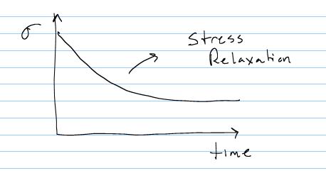
The ability to dissipate energy is one of the main reasons for using viscoelastic materials for any application to cushion shock, from running shoes to packing materials. The two other main characteristics associated with viscoelastic materials are stress relaxation and creep. Stress relaxation refers to the behavior of stress reaching a peak and then decreasing or relaxing over time under a fixed level of strain, as shown below:

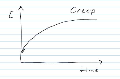
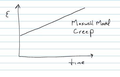
Creep is in some sense the inverse of stress relaxation, and refers to the general characteristic of viscoelastic materials to undergo increased deformation under a constant stress, until an asymptotic level of strain is reached, as shown below:

Any materials that exhibit hysteresis, creep or stress relaxation can be considered viscoelastic materials. In comparison, elastic materials do not exhibit energy dissipation or hysteresis as their loading and unloading curve is the same. Indeed, the fact that all energy due to deformation is stored is a characteristic of elastic materials. Furthermore, under fixed stress elastic materials will reach a fixed strain and stay at that level. Under fixed strain, elastic materials will reach a fixed stress and stay at that level with no relaxation.

III. Mechanical Analogs for Viscoelastic Materials

      The classic description and way to derive viscoelastic consitutive models is through the use of mechanical analogs. These are simple mechanical models for fluid and solid representations that are put together to produce viscoelastic effects. The simplest mechanical analog for a linear elastic material is a spring:

The simple constitutive relationship for a spring relates the force (and stress by extension when force is divided by area) to the elongation or displacement (and strain by extension when displacement is normalized by length of the spring):

where Fs is the spring force, E is the elastic modulus of the spring, and us represents the spring displacment. The mechanical analog for a Newtonian fluid is a dashpot. The simple constitutive relationship for a dashpot indicates that the force in the fluid depends on the rate the dashpot is displaced, or equivalently the velocity of the dashpot.

Also, the constitutive parameter that relates force (stress) to displacement rate (strain rate) is viscosity, which we denote as m. Thus, the constitutive equation for a fluid may be written as:

where the dot over the u in the equation indicates differentiation with respect to time and the superscript d denotes "dashpot".

By making various combinations of spring and dashpot models, we can simulate the behavior of a viscoelastic material, including stress relaxation and creep.

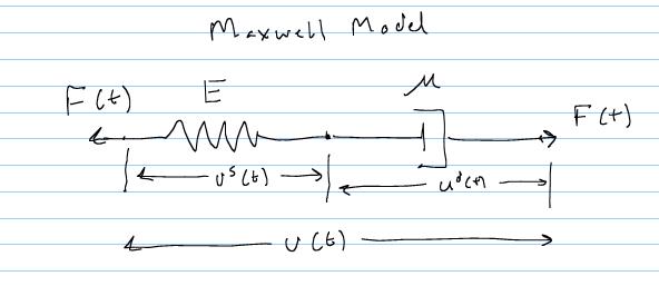
The simplest combination of the spring and dashpot is to put the spring in series with the dashpot:

 

This combination is known as the Maxwell model. As we will see, this model actually represents a fluid since it relaxes completely to zero stress and undergoes creep indefinitely. To derive the constitutive relation, we note first examine the kinematics of the model. It is clear from the geometry of the model that the total displacement will be the spring displacement plus the dashpot displacement:

However, the constitutive displacement for the dashpot is written in terms of the dashpot displacement differentiated with respect to time. Thus, to be consistent, we will differentiate the above expression for the total displacement with respect to time. This gives:

We need to determine both the displacement rate for the solid and the fluid. For the fluid, we simply rearrange the fluid constitutive equation:

To get the solid displacement rate, we first rearrange the constitutive equation for the spring:

we then differentiate this constitutive relationship with respect to time to obtain:

since E does not depend on time. Putting these together we get the total displacement rate as:

By normalizing the force by area and the displacement by length, we can get the analogous stress-strain relation as:

were the s and d superscripts have been dropped. We also have the following dimensions for the spring constant E and the viscosity m:

If we assume constants q1, p0 and p1, we can rewrite the above equation as:

where the constants are defined as:

Now, let us consider the behavior of a Maxwell material under conditions of both fixed strain and fixed stress. We assume that strain and stress can be applied instantaneously to a fixed level. In reality, instantaneous stress or strain cannot be reached, but we assume that in the limit, for example, if the test is run long enough, that the stress or strain can be considered to be reached instantaneously. We start with the response to an instantaneous strain that is then held constant over time:

In this case, the rate of change of strain is zero. Thus the equation for the Maxwell material becomes:

To solve for the stress under fixed strain for a Maxwell material, we need to solve the ordinary differential equation in time. To do this, we can again use the symbolic toolbox in MATLAB. First, we divide through by p1 to obtain:

We can then use the dsolve option in the MATLAB symbolic toolbox to solve the ordinary differential equation in time. The differential equation is put in parentheses after we define the symbols:

>> syms sig
>> syms sig p0 p1
>> dsolve('Dsig + (p0/p1)*sig = 0')

ans =

C1*exp(-p0/p1*t)

MATLAB returns a constant C1 which is an integration constant. We can write the equation as:

To solve for the integration constant C1, we need to determine the initial condition at time t = 0+ on the stress. To do this, we need to integrate the Maxwell constitutive equation from time t = 0- to some short time t = tn just after the strain is applied:

The integration gives us:

we know that e at t = 0- is 0 and e at t = tn is e0. Also, s at t = 0- is 0 and s at t = tn is s0. For the last term, we assume that tn is a small number. As we keep ramping up in shorter and shorter times, in the limit we approach tn = 0+, a nearly instantaneously applied strain. In this case,

This means the last term in the integration is zero and we are left with:

Thus, if we substitute in the initial condition to the solution of the Maxwell model constitutive equation we obtain the constant C1:

Thus, we have the general solution for the Maxwell model under a step strain as:

or if we write the constants in terms of the spring modulus and dashpot viscosity:

Now if we divide the stress as a function of time by the initial strain, we obtain the stress relaxation function G(t) for the Maxwell model:

This is a characteristic function that tells us how the stress relaxes for a given material. If we plot the the stress relaxation versus time we obtain the general curve:

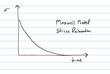
Note that the stress completely relaxes out over time. This is actually characteristic of a viscoelastic fluid rather than a viscoelastic solid. Finally, we note that the ratio m/E gives us a dimension of time. This is a characteristic time of the material denoted as the relaxation time, and defined as:

Using the relaxation time, we can rewrite the relaxation function as:

Now let us consider the response of the Maxwell model to a unit step stress:

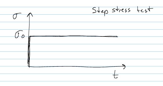
In this case, a stress s0 is applied "instantaneously" and then kept constant over time. Thus, the rate of change of stress is zero and the Maxwell constitutive model becomes:

We can solve the above equation simply by integrating with respect to time. We can also do this in MATLAB as:

>> syms eps sig0 p0 q1
>> dsolve('Deps = (p0/q1)*sig0')

ans =

p0/q1*sig0*t+C1

or:

where again C1 is a constant of integration that we need to determine from initial conditions. Given the initial conditions derived before, we obtain:

This gives the strain versus time under a unit step stress as:

Similar to the stress relaxation, we can define a creep function J(t) by dividing the strain versus time reponse by the initial unit step stress. This gives the creep function Jas:

Note that the above equation will give a constantly increasing strain as a function of t:

This is also not characteristic of a viscoelastic solid, since we expect that the creep will reach an asymptotic level after a certain time.

Although the Maxwell model did not give us a realistic result for a viscoelastic solid (it is more representative of a viscoelastic fluid) it did allow us to illustrate some important aspects of a viscoelastic material including the stress relaxation function G(t) and the creep function J(t). We next consider another mechanical analog for a viscoelastic material, the Voight model, also known as the Kelvin-Voight model. Its geometry is shown below:

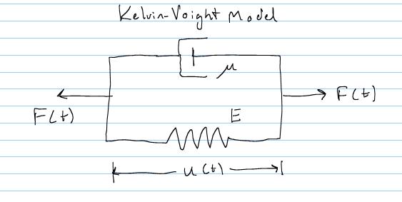
Again, we can make observations based on the geometry of the model. First, we note that the dashpot will constrain the spring to have the same deformation:

Second, we note that the total force F in the Voight model will be equal to the force in the dashpot plus the force in the spring:

We can substitute the force-displacement relationship for the spring, and the force displacement relationship for the dashpot to give:

By analogy, we can write a stress-strain differential equation as:

The above equation again illustrates an important characteristic of viscoelastic materials, namely that the stress in the material depends not only on the strain, but also on the strain rate.

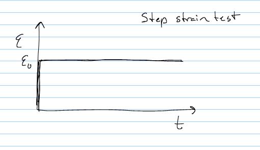
Let's now see how the Voight model responds to a unit step stress and strain. First, we consider the unit step strain again:

For this step strain, we again need to integrate the Voight constitutive equation to obtain the initial conditions:

For the last term in the integral, we have:

For the second term, we have:

If we look at the first term, it will give us the area under the stress versus time curve. This area must have a limit, otherwise we would have infinite stress. Thus, in the limit as the time becomes very short, the area must have a finite value. This is given by the dirac delta function (not to be confused with the kronecker delta), which has the property:

Thus, we have the following initial condition for a step strain test:

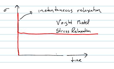
which gives us the following stress versus time response:

This gives a stress relaxation function as:

This function gives instantaneous stress relaxation due to the presence of the dashpot.

Next, let us consider the response of the Voight model to a unit step stress:

We again solve the differential equation in time for the Voight model using MATLAB. To get the equation into a form we can use for MATLAB, we first divide through by the viscosity and recognize that the stress is constant s0 to get:

We can then solve this equation in MATLAB:

>> syms sig0 eps emod mvis
>> dsolve('Deps + (emod/mvis)*eps = sig0/mvis')

ans =

sig0/emod+exp(-emod/mvis*t)*C1

or, in other words:

where again C1 is a constant of integration. To determine the constant C1, we again need to use the initial condition. In this case, under an instantaneously applied stress, the dashpot cannot move instantaneously. Thus, this means that there will be no displacement and therefore the strain at time t = 0 will be zero. Pluggin this initial condition into the above equation gives:

This give us the solution:

If we divide the above by s0, we obtain the creep function J:

The above function gives us a strain versus time plot as shown below:

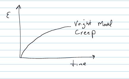
Note that no instantaneous elastic deformation is possible due to the restraint of the dashpot.

Note that if we rearrange the above equation we can write the strain as a function of time and the initial stress as:

Note that as mentioned before the dashpot does not allow instantaneous deformation to occur, but overtime the displacement creeps to an asymptotic level.

IV. Generalized Viscoelastic Constitutive Models

      We can see from the mechanical analogs investigated in the previous section that the strain behavior over time of a viscoelastic material is a function of the creep function and the stress, while the stress behavior over time is a function of the stress relaxation function and the strain. Boltzmann (1844-1906) first generalized these observations by saying that for a simple bar subject to a stress s(t), that the increment in stress over a small time interval dt would be:

This assumes that the stress is continuous and differentiable in time. Given that the stress is related to the stress via the creep function, Boltzmann postulated that an increament of strain de, which depends on the complete stress history up to time t, would be related to the increment of stress ds at the specific time increment from t to t through the creep function J at the time t - t as:

The complete strain at a time t would then be obtained by integrating the strain increments from time 0 to time t, over all the increments dt:

We can also make the same argument for an increment of stress ds through time t depending on the increment of strain de at time t and the stress relaxation over the time t - t as:

Again, if we integrate over the entire strain history we obtain:

The above constitutive relationships can be generalized to three dimensions in tensorial form for a strain history from time t = - infinite to t as:

where now there is a tensorial stress relaxation function Gijkl.

We can write a similar relationship for strain in terms of a prescribed stress history and a tensorial creep function Jijkl as:

If we know that the loading starts at t = 0 and the stress and strain are zero at this point, we may write the above constitutive relationships as:

and

V. Fung's quasi-linear viscoelasticity theory

      The constitutive equations presented in the mechanical analog section and the generalization seen above work for materials undergoing small strain. However, we have seen that most soft tissues undergo large deformation. To account for this, Fung (see Y.C. Fung, Biomechanics: Mechanical Properties of Living Tissues) introduced the concept of quasi-linear viscoelasticity (QLV) theory. In this case, Fung introduced a separation of the stress relaxation function into a time dependent part and an elastic portion. This gives:

where now the total stress relaxation function K depends on both time and the stretch ratio l in terms of a reduced relaxation function G that only depends only on time and an elastic response Te that depends on the stretch ratio. In this way, the theory is linear in the relaxation response but still accounts for nonlinear large deformation.

The stress response for an infinitesimal change in stretch can then be written as:

where T is the 1st PK stress as a function of time, and Te is an energy function. If we assume that superposition holds for the linear case, we can integrate the above equation to obtain:

Note that the form above is very similar to the linear viscoelastic model for stress, with Te the elastic response depending on the stretch ratio replacing the small strain rate.

Fung also proposed a general stress relaxation function for use in QLV. This reduced relaxation function is given as:

where c is a constant, t1 and t2 are characteristic times during relaxation, and E1 is the exponential integral:

note that as t goes to inifinity the above integral goes to zero and the reduced relaxation function reduces to:

QLV is an approximation used quite often for viscoelastic constitutive models of soft tissues.

VI. Example of Computing Stress Versus Time for a Quasilinear Viscoelastic Model

       To give an example of a quasilinear viscoelastic model, consider the model proposed by Toms et al. (2002) in the Journal of Biomechanics for periodontal ligament. The periodontal ligament is a thin piece of soft tissue interposed between a tooth and the surrounding alveolar bone. The PDL provides cushioning between the tooth and the bone, as well as being a conduit for nutrients. It is also known that the mechanical behavior of the PDL is nonlinear and viscoelastic. To characterise this behavior, Toms et al. chose to use the quasilinear viscoelastic approach of Fung, where the general constitutive equation is represented by:

although they did not use the reduced relaxation function proposed by Fung. Instead they chose a general decaying exponential function of the form:

where e is the exponential function, t is time, and a,b,c,d,g,h are all coefficients to be determined by experiment. This was a function that had been previously proposed by Will et al. in 1972 for characterising the viscoelastic behavior of the PDL. For the instantaneous nonlinear elastic response, Toms et al chose a very commonly used form:

where T is the 1st PK stress, e is the exponential function, l is the principal stretch ratio, and A and B are constants to be determined experimentally. The strain energy function that would correspond to this instantaneous nonlinear elastic response can be derived by integrating the 1st PK stress over l. We can do this quite easily using the MATLAB symbolic toolbox as follows:

As always, we first define the symbols we will be using:

>> syms A B lam

We then perform the integration in MATLAB using the int command, where we specify the function followed by l as the variable of integration:

>> int(A*(exp(B*lam)-1),lam)

The answer is:

ans =

A*(1/B*exp(B*lam)-lam)

which gives the strain energy function defined as:

Thus, the elastic response becomes the second derivative of the strain energy function with respect to the principal stretch ratio which gives us the 1st PK stress.

Let's consider a ramp displacement of the PDL with the following time constant:

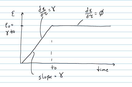
Now let us calculate the 1st PK stress at some time past t0. To do this, Toms et al used the following test set up to determine the nonlinear elastic response as well as the time dependent stress decay:

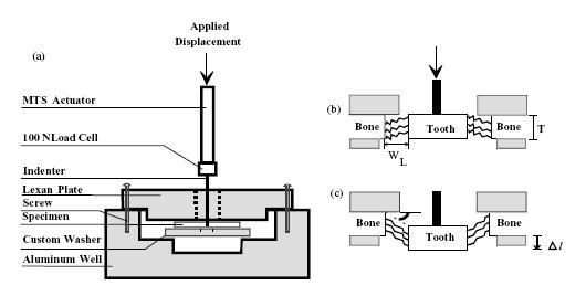
which was used due to the thinness of the PDL and the difficulty in separately the PDL from the tooth and the alveolar bone. Based on Toms results, let's calculate a typical stress time reponse analytically. To do this, we write the general form of the quasilinear viscoelastic function:

where E is the large strain tensor. For the above ramp strain, we know that the strain rate after t = t0 is zero since the strain is constant. Therefore, we need only integrate to t0. Furthermore, we know that the strain rate up to t0 is a constant g, which we can substitute into the above equation to obtain:

we can now integrate a general expression for the 1st PK stress analytically in MATLAB, in similar fashion as to how we integrated the stress to get the strain energy function. We first define the symbols:

>>syms a b c d g h A B lam t tau t0 gam

we next write the function and integrate the function over t from 0 to t0:

>> int(A*gam*(exp(B*lam)-1)*(a*exp(-b*t+b*tau)+c*exp(-d*t+d*tau)+g*exp(-h*t+h*tau)),tau,0,t0)

MATLAB gives us the answer:

ans =

A*gam*(exp(B*lam)-1)*(a*exp(-b*t+b*t0)*d*h+c*exp(-d*t+d*t0)*b*h+g*exp(-h*t+h*t0)*b*d-a*exp(-b*t)*d*h-c*exp(-d*t)*b*h-g*exp(-h*t)*b*d)/b/d/h

or written out:

Now let us use the above analytical expression to compute stress versus time. We first enter values for all the constants in MATLAB:

>> a=.0856;
>> b=.154;
>> c=.08;
>> d=.002;
>> g=.8244

g =

0.8244

>> h=1.25e-5;
>> h

h =

1.2500e-005

>> A=8.92e-3;
>> B=8.79;
>> lam=1.3;
>> 0.5*(lam^2-1)

ans =

0.3450

>> t0 = .345/4.

t0 =

0.0862

>> gam=4.;

Note that these values are made up.

Next, we generate a time array going from 0 to 86 seconds:

>> t=[1:1000]*.0862;

Finally, we generate the for loop that computes stress as a function of time:

>> for i = 1:1000
sig(i)=A*gam*(exp(B*lam)-1)*(a*exp(-b*t(i)+b*t0)*d*h+c*exp(-d*t(i)+d*t0)*b*h+g*exp(-h*t(i)+h*t0)*b*d-a*exp(-b*t(i))*d*h-c*exp(-d*t(i))*b*h-g*exp(-h*t(i))*b*d)/b/d/h;
end

We can now plot stress from time t = t0 to a longer time t. We obtain the following curve:

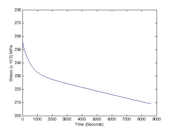
We see that the stress relaxes fairly quickly after an initial ramp up.

 

 

VI. Summary