I. Overview

       In the last section we introduced some basic ideas of biphasic theory and poroelasticity for modeling tissues as fluid filled solids. The purpose of this section is to illustrate how constants for the linear biphasic theory may be fit for creep and stress relaxation experiments. In this case, our approach will follow those for fitting nonlinear elastic and quasi-linear viscoelastic theory. We will propose an experiment, derive the stress and deformation from that experiment, derive stress from the proposed constitutive model, and then use optimization to fit constants by solving the equilibrium equations for the proposed experiment.

II. Review of Linear Biphasic Theory

      In this section we will review the basic tenets of linear biphasic theory. The basic idea of biphasic theory is that a material or tissue is composed of a fluid phase and a solid phase, hence the name "bi" (two) phasic. In biphasic theory, we need to address the fact that both mass and momentum are conserved within each phase. Mass cannot be created or destroyed in either phase. The continuity equations govern this stating that the net flux of mass is zero. These are written separately for the solid and fluid phase as:

     

    

where rs and vs denote the density and velocity of the solid phase and corresponding variables with f superscripts denote the density and velocity of the fluid phase. These equations simply state that within the solid and fluid phase that the time rate of change of density and the gradient of the change in density within the 3D space must be zero. Likewise, we also have to satisfy conservation of momentum within each phase. However, where the two phases meet, we also have to account for the fact that we have the fluid phase particles interacting with the solid phase particles. As these particles interact with the fluid phase moving relative to the solid phase, there is a force that is created due to this interaction which we call a drag force and denote with p. Therefore, accounting for drag forces between the fluid and solid and the inertia forces we have the following equilibrium equations for each phase:

     

     

where the new variables are the solid stress ss, the solid drag force ps and the corresponding fluid stress and drag force denoted with a superscript f. These are the governing equations for a biphasic tissues.

If we look at the continuity equation, we can make the following arguments. First, the density of the solid phase is given per unit of the mixture. If we denote the density of the solid phase per the solid phase as:

Then the density per the unit mixture is simply the volume fraction of the solid phase times the density of the solid phase rendered per the solid phase. Denoting the solid phase volume fraction (that is, how much of the total mixture is a solid) as fs, we have:

We also note that the volume fraction of the solid plus the volume fraction of the fluid phase must add up to one:

We can rewrite the continuity equations as:

Where we assume the initial phase density is homogeous (for example, the solid phase is homogeneous through that phase. If we note from the requirement that the fluid and solid phases add up to one and substitute this into part of the fluid equation we have:

If we add these two equations we are left with:

In summary, the governing mass and momentum conservation equations for the biphasic theory are:

Next, of course, we need to propose a constitutive model for both the fluid and solid phases. For both phases we assume incompressiblility. For the solid phase, we assume linear elasticity with the incompressibility assumption giving:

which for the isotropic case becomes:

for the fluid phase we have:

For the 1D linear isotropic elastic case we have:

The solid stress may be further written in terms of an aggregate modulus and the unixaxial strain as:

If we combine the 1D linear elastic isotropic constitutive model with momentum and mass balance equations we have:

If we solve for the pressure from the fluid equation and substitute this into the solid equation we obtain:

 

To further reduce this equation, we need to consider the mass conservation equation:

If we integrate this equation, we get an integrating factor v0 which is an initially applied velocity as:

Substiting this result into the 1D momentum balance equation and noting that the fluid and solid volume fraction must add up to 1:

 

For most tests, the initial velocity is zero, therefore, v0 may be eliminated. Finally, we note that the drag coefficient K is actually equal to the volume fraction of the fluid square divided by the initial permeability k0. This leaves us with:

 

The final 1D linear equation for biphasic theory that may be used to analyze both stress relaxation and creep is given by:

where u3 is the displacement in the z direction, Ha is the aggregate modulus defined as:

and k0 is the intrinsic permeability of the material.

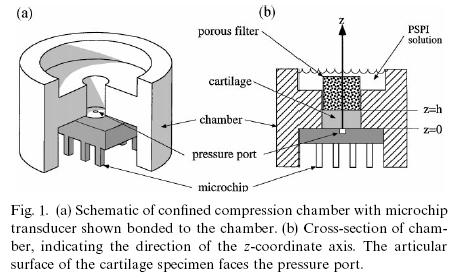
To solve this time dependent 1D partial differential equation, we need to know both initial conditions and boundary conditions. In the typical 1D test performed on biphasic tissues, one side of the tissue is next to an impermeabile platen, and the other "z" side of the tissue next to a permeable platen, with the sides of the tissue constrained, as shown in the schematic below from Soltz, MA and Ateshian GA, "Experimental verification and theoretical prediction of cartilage intersitial pressurization at an impermeable contact interface in confined compression", J. Biomechanics, 31:927-934, Figure 1:

The boundary conditions under this test are such that no tissue displacement occurs at the rigid platen interface, and thus:

which means that u3 at x3 = 0 is zero for all time t during the test. The initial conditions are such that the displacement through all the tissue is zero at the intial time t = 0, and thus this is the initial condition:

If we are performing a creep test on a biphasic specimen, a ramp force is applied at the top surface of the cartilage specimen where x3 = h. Thus, the boundary conditions at the top of the specimen are:

For the 1D partial differential equation (PDE), Soltz and Athesian derived the following solution under the boundary conditions above:

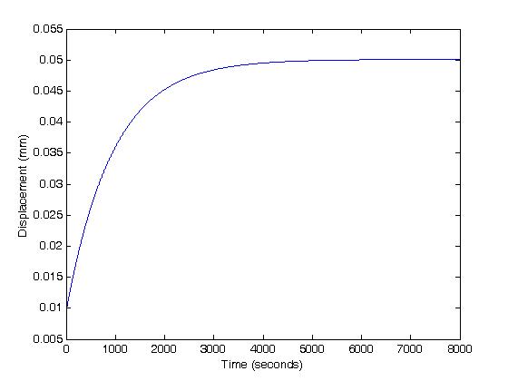
To better see how the solution behaves, let's consider the displacement at the surface (x3 = h) and use only the n = 0 term for the sum. Then the above becomes:

or

If we plot the displacement for this function as below:

t=0:8000;
>> for i = 1:8001
u3(i)=-(pa/ha)*(h-.8106*h*exp(-2.468*ha*k0*t(i)/h^2));
end
>> plot(t,u3)

we obtain:

 

III. Plotting Biphasic Creep in MATLAB

      As a precursor to doing the optimization in MATLAB, we will again perform a plot of the solution for the given parameters. From the Soltz and Athesian paper we have the following constants:

h = 0.81mm

HA = 0.97 MPa or N/mm^2

K0 = 2.9 x 10^-16 m^4/Ns or 2.9x10^-4mm^4/Ns

PA=-0.06MPa

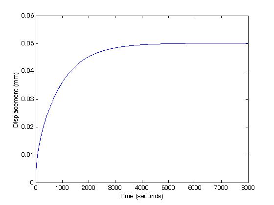
We can write a simple MATLAB command line to plot the results for time t up to 8000 seconds:

>>t=0:8000;
>> u3=zeros(1,8001);
>>for i = 1:8001
a = 0.0;
for n = 0:100
a = a + ((-1)^n/((n+0.5)^2))*sin((n+0.5)*pi)*exp((-ha*k0/h^2)*pi*pi*t(i)*(n+0.5)^2);
end
u3(i) = -(pa/ha)*(h-(2*h/pi^2)*a);
end

When we do this, we get the following creep plot:

III. Optimization to Fit Biphasic Constitutive Parameters in MATLAB

      Once we have an analytical solution for the creep response of a 1D biphasic material, we can then perform optimization to fit the biphasic parameters to experimental data. In this case, the experimental data will be the time dependent creep displacement. The two parameters we will fit in the 1D case are the aggregate modulus Ha and the permeability k0. This procedure again follows the same general outline the we have used to fit nonlinear elastic and quasi-linear viscoelastic constitutive parameters. This schematic is shown below:

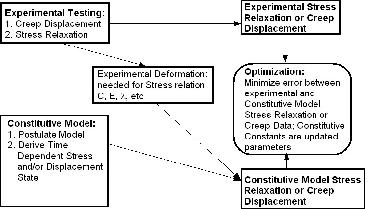
In this case, however, we will be matching creep displacement data, not stress data. Since we do not have any constraints, we will initially use the fminunc, nonlinear minimization without constrains, function in MATLAB. Recall that we again need to write a MATLAB function to evaluate the objective function in terms of the current constant parameters. Such a function is given below:

 

Please note that I have essentially generated the experimental data from the analytical solution provided by Solz and Atheshian. To call the optimization function, we use the following commands in MATLAB:

 

>> cf=[1 1]
>> cf0=[1 .001]

[c,fval,exitflag]=fminsearch('biphasicfitun',c0)

 I have used fminsearch, an unconstrained optimization routine, for this problem as it seemed to give a better results. If we choose these starting points, then we obtain the coefficients:

cf =

0.9701 0.0003

fval =

3.2895e-010

Note that this is basically the same result as obtained by Soltz and Athesian. However, this is somewhat cheating since we know the desired outcome. Let us choose a standard starting point of cf =[1 1].

We obtain:

cf =

1.0617 0.8568

fval =

0.0024

Note that the results are much different, but that the objective function is much smaller with the actual solution. Plotting both results, however, clearly shows that the solution given the initial guess of 11 is not satsifactory:

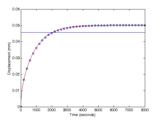
where the stars are the "experimental" data, the red line is the optimization solution for the "good" guess, and the dark line is the optimization solution for the typical guess. This points to a significant problem in that we clearly need to know something about the physical behavior of the cartilage to guide us in the solution. One thing we do know is that cartilage has a very low permeability, typically much less than .001 mm^4/Ns. Therefore, we can try this as an upper bound on the permeability in fmincon. This is done as:

>> [cf,fval,exitflag]=fmincon('biphasicfitun',cf0,[],[],[],[],[],[1000.,.001])

where now we create an array with upper bounds of [1000,.001]. We have chosen an abitrarily large value for the aggregate modulus. The results give us the "correct" solution of:

> In fmincon at 260
Optimization terminated: magnitude of directional derivative in search
direction less than 2*options.TolFun and maximum constraint violation
is less than options.TolCon.
No active inequalities

cf =

0.9701 0.0003

fval =

9.9534e-009

VI. Summary

       This section shows how we can determine coefficients for the 1D biphasic theory for articular cartilage, assuming the solid matrix is isotropic linear elastic. The results, however, bring up a word of caution. We cannot blindly apply the optimization routine, but need to know something about the range of physical properties. This allows us to put bounds on the solution using the fmincon solver in MATLAB. The resulting solution with bounds gave us the correct solution. Another important point raised in the biphasic constant fitting is that even for the experimental solution we need actually to solve a partial differential equation to obtain the experimental displacement or stress data. In the nonlinear elastic case for heart muscle, the partial differential equation was bascially a trivial situation in which we could ascertain the correct solution by physical reasoning. This is not, however, often the case.