BME 456: Biosolid Mechanics: Modeling and Applications
Section 3: The Concept of Deformation and Strain
I. Overview
In the last section we derived the stress equilibrium equations based on considerations of force balance within the material. The stress equilibrium equations, although derived for the deformed state of that material, did not entail any assumptions about the material or the type of deformation it encurs. We learned that for most situations, the stress equilibrium equations are indeterminate, and we can't solve for material stresses directly from these equations. We therefore need to consider other aspects of the material and tissue mechanics. The next logical step is to examine then how the material deforms. It is at this point that we introduce our first significant assumptions concerning continuum mechanics. If we make no assumptions about the size of deformation, then the resulting strain tensor is valid for every situation. However, this strain tensor is nonlinear and leads to complex analysis. Therefore, if the deformation is small (typically less than 3-4%), then we can use a small deformation analysis, which is linear and simpler to use. In tissue mechanics, hard tissues fit under the small deformation model, but most soft tissues typically undergo large deformation (strains > 5%). In this section, we will discuss and derive deformation and strain measures for both small and large deformation. By the end of this section, you should be able to:
1. Understand concepts of the small deformation tensor
2. Understand concepts of initial and deformed configuration
3. Understand the concept of displacement
4. Understand the concept of the deformation gradient tensor
5. Understand the concept of the large deformation strain tensor
6. Understand differences between small and large deformation
II. Small Deformation Strain Tensor
We first consider the case of small deformation, since this is applicable to bone and is much less complex than large deformation. Consider the deformation of an infinitesimal cube (once more!) in the x1 direction:
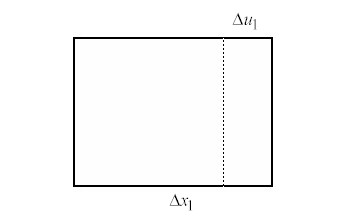
We know that if the displacements are small, then we can approximate the normal strain in the 11 direction as:
If we in the limit allow both ![]() and
and
![]() both to approach
zero, then we arrive at the following strain displacement relationship:
both to approach
zero, then we arrive at the following strain displacement relationship:

This corresponds to our notion that strain is defined as the change in length over length. Note that this is an approximation of strain for small deformations. Thus, it is our definition of strain that renders this discussion for the small deformation part of small deformation elasticity. We can also do the same change in length for the x2 and x3 directions to arrive at:
Next, let us consider a pure shear deformation as shown as the infinitesimal cube below:
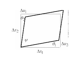
Here, the total deformation is the sum of the angles q1 and q2, and can be written as:
Note that q1 is defined to equal q2,q1 = q2. Now we use some trigonometry. We note that the tangent of q1 and the tangent of q2 can be written as:
If we assume that the angle of deformation is small (again referring back that this section is small deformation strain), we know that the tangent of a small angle is equivalent to the angle itself, assuming we define the angle in radians. Thus, we may write the above as:
We can thus rewrite the angular deformation from above as:
Note that we have added an extra definition e12. This is the definition of tensorial shear strain that is one half g12 that is the definiton of engineering shear strain. If we taken the limit as all delta quantities go to zero, then we have the following definition of the shear strain:
by definition shear strains are symmetric as we see below:
The definition of the other shear strains follows directly as:
Given the definition of normal strains, and the shear strains given above, we can write a compact defintion of small strain in indicial notation as:
Note that the small deformation strain is a second order tensor just like the Cauchy stress tensor. It has nine components for 3D. We can write the small deformation strain tensor in matrix form as:
How does the addition of the strain displacement relationship affect our ability to solve the mechanics problem. Well, now we have introduced 12 more unknowns, the nine strains eij and the three displacements ui. We have introduced, however, only 9 additional equations, namely the strain-displacement equations.
III. Definition of Reference and Deformed Configurations, and the Relationships between Them
We explicitly made the assumption in deriving the small strain tensor that strains were "small" for both normal and shear strain. While this assumption is valid for bone, it is not valid for soft tissues. Of course, one may ask why bother with assuming small deformation at all. As we will see in this section, large deformation, while valid for all deformation situations, is much more complex and introduces nonlinearity into the problem, called geometric nonlinearity.
III.A. Reference (Initial) and Deformed Configurations
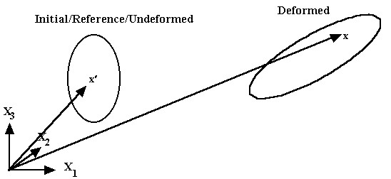
The first step in defining large deformation strain measures is to define the relationship between what is known as the reference, initial or undeformed configuration of a body, and the deformed configuration of the body. The reference or undeformed configuation is the condition of the body in 3D space before loads have been applied to it. The deformed configuration is the location and shape of the body after loads have been applied to it. It is important to note that the body may undergo rigid body motion in addition to strain when loades are placed on it. An illustration of the relationship between the initial (note that I will use initial, reference, and undeformed configuration interchangeably throughout this section) and deformed configuration is shown below:
III.B. Displacement: Relationship between a point in the Reference and Deformed Configuration
Note that we have defined a vector in 3D space x' in the reference configuration of the body and a vector x in the deformed configuration of the body. We note that the relationship between the two position vectors in space, which represent the locations of a point in the reference configuration and a point in the deformed configuration, is the displacement vector, as shown below:
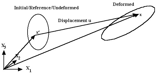
By vector addition, we can directly write the relationship between the position vectors in the initial and deformed configuration:
III.C. Deformation Gradient: Relationship between a material vector in the Reference and Deformed Configuration
The above results tells us how a point displaces from the reference to the deformed configuration. However, we would also like to know how a piece of material, again, an infinitesimal piece, is stretched and rotated as the body moves from the reference to the deformed configuration. The infinitesimal material vector in the reference configuration, dx', is shown in red in the reference configuration. The material vector after it has been stretched and rotated, dx, is shown in red in the deformed configuration below:
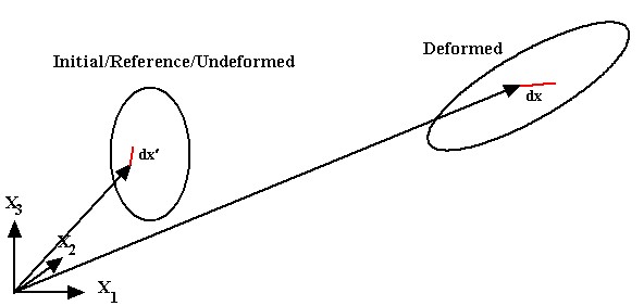
Since the length of dx' can change when going to the deformed configuration as well as its orientation, we can say that dx' deforms into dx. The question then becomes how to relate dx in the deformed configuration into dx' of the reference configuration. This can readily be done through the chain rule as:
The above equation gives a relationship between a material vector in the undeformed and deformed configuration. We define the mapping itself as the deformation gradient tensor:
 .
.
where Fij is the deformation gradient tensor. We know by the rules of index notation that F is a second order tensor, since it has two independent indices. It is also important to note that F IS NOT Symmetric. We can also write the deformation gradient tensor in matrix format as:
III.D. Relating the Displacement Vector and Deformation Gradient Tensor
We now have two entities that relate quantities in the reference configuration to the deformed configuration: the displacement vector and the deformation gradient tensor. The next logical question is whether these quantities themselves have any connection. First, let us begin with the displacement vector that relates a position in the reference configuration to a position in the deformed configuration:
![]()
The above equation actually represents the relationship between the three coordinates in a reference and deformed configuration:
Now let us differentiate each on of the above equations with repect to
![]() ,
, ![]() ,
and
,
and ![]() :
:
Let's first look at and group the left hand side of the differentiated displacement relationship. If we group all these terms, we end up with the deformation gradient tensor. Now, let's take a look at the first term on the right hand side in each of the above equations. If we group these terms in a matrix, we obtain:
Let us look more carefully at each entry in the above matrix. Obviously, if we differentiate something with respect to itself we get 1. Thus, the diagonal of the above matrix will all have ones. For all the off axis terms, we are differentiating a one coordinate position with respect to one of the two other coordinate positions. Since one coordinate position (e.g. 1,2,3) does not depend on the other coordinate positions, these terms are all zero. This leaves us with the identity matrix, which is equivalent to the kronecker delta 2nd order tensor we defined in the section on mathematical preliminaries:
Finally, we consider the term on the right hand side of the differentiated displacement equation. We can also write this in a matrix from as:
We can also recognize from the mathematical preliminary section that the
above entity is the
gradient of the displacement. We can therefore recognize that differentiating
the displacement equation with respect to ![]() ,
,
![]() , and
, and
![]() gives
us the deformation gradient tensor being equal to the kronecker delta second
order tensor plus the graident of the displacement. This relationship is
written in both matrix and index notation below:
gives
us the deformation gradient tensor being equal to the kronecker delta second
order tensor plus the graident of the displacement. This relationship is
written in both matrix and index notation below:
Matrix Notation:
Index Notation:
III E Decomposing the Deformation Gradient Tensor in Stretch and Rotation Tensors
As we noted earlier, the deformation gradient tensor includes both rigid body and deformation modes. Therefore, we should be able to decompose the deformation gradient into rigid body and deformation components. Since translation does not change any vector or its components, we can therefore conclude that the deformation gradient tensor contains only deformation plus rotation components. To verify this, consider pure translation. In this case, we may write directly x in terms of x' plus a translational component:
If we plug the above translation component into the deformation gradient tensor definition we have:
In pure translation, all points in the body will move the same amount in each of the three orthogonal directions. This means that s1, s2, and s3 will not differ at different points in the body. Thus, the gradients of s1, s2 and s3 with respect to x' will all be zero. This leaves us with the fact that the deformation gradient tensor is the identity under pure translation:
we also not that when there is no displacement at all the deformation gradient tensor will also be equal to the identity tensor. Thus, the deformation gradient tensor does not distinguish between states of translation.
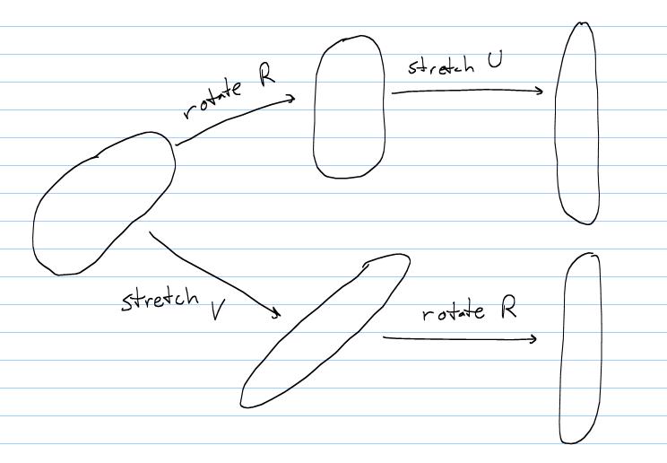
Thus, we know that the deformation gradient tensor will only contain the rigid body mode of rotation in addition to stretch. We therefore postulate without proof that the deformation gradient tensor can be decomposed into a rotation multipled by stretch or a stretch multiplied by rotation. Let us denote the rotation tensor by R. If we decompose the deformation gradient tensor such that we rotate first and then stretch, we denote this stretch tensor by U. We therefore can write this decomposition as:
![]()
If we first stretch and then rotate, we denote the stretch tensor by V, and can write the decompositon as:
![]()
Graphically, we can represent this decomposition as:
We further note that the rotation tensor has special properties, namely that it is orthogonal. This means that the transpose of the rotation tensor multiplied by itself will give the identity tensor:
![]()
This property will play a role in the definition of other deformation tensors, which themselves play a significant role in definition of many constitutive equations.
IV. Definition of Large Deformation or Finite Strain Tensor and other Deformation Tensors in terms of the Deformation Gradient Tensor
Once we have defined reference configuration, deformed configuration, displacement, and deformation gradient tensor, we can derive the large strain tensor. We cannot use the deformation gradient tensor as a strain measure directly because it can contain rigid body modes like translation and rotation. For a strain tensor, our goal is to obtain some measure the change in length of a material. One way to measure length is to take the dot product of the material vector we used when defining the deformation gradient with itself. Thus, the length squared ds'^2 of the material vector in the reference configuration is:
![]()
We can likewise write the length squared of the material vector ds^2 in the deformed configuration as:
![]()
The strain tensor should be a measure of how much the material vector in the reference configuration is stretched into the deformed configuration. We would essentially like the strain measure to operate on the material vector in the reference configuration and generate the difference in the square of the lengths of the material vector. We may write this idea in compact index notation as:
Note that the above equation represents the difference two scalars, the square of the length of material vectors in the reference and deformed configuration. If we expand this equation we can see this more clearly:
Note that E, which will be defined as the large deformation or finite strain tensor, has 9 components in 3D making it a 2nd order tensor. Two thirds of the strain equation above is written in terms of dx'. Therefore, to define Eij we will need to write the square of the length of the material vector in the deformed configuration also in terms of the reference configuration vector dx'. One way we can do this is to use the deformation gradient tensor, which gives the material vector dx in the deformed configuration in terms of the material vector dx' in the reference configuration. We also need to write the relationship using the deformation gradient tensor such that we obtain pre and post multiplication by dx'i and dx'j, respectively. First, since the quantity dxidxi is a scalar with repeated or dummy indices, it doesn't matter if we write the repeated index with i,j,k, or any other letter, it will produce the same result. So, let us write the dot product with a k:
![]()
Next, we can write the deformed configuration material vector in terms of the deformation gradient tensor and the reference configuration material vectors as:
![]()
This gives us the dx'j post multiplication term. Note that if we change the order of F and dx', this will not change the result. Also, since j is a repeated or dummy index in the above equation, we can replace it with any other repeated index, including i. If we carry out these operations, we obtain:
![]()
Just to show that the Fkjdx'j and the dx'iFki give equivalent expressions,
we will expand each expression. For ![]()
For ![]() we have:
we have:
we can see that the two above equations are equivalent. We can now substitute the expressions with the deformation gradient into the strain equation to obtain:
![]()
The last task in defining Eij is to somehow rewrite the dx'idx'i term as a dx'idx'j term. To do this, we can simply apply the Kronecker delta as:
![]()
We can expand the above relationship as:
which shows that multiplying by the kronecker delta gives us back the original quantity. We can now substitute in for the kronecker delta term into the large strain equation to give:
![]()
We note that the above relationship can be separated in terms of dx'i as:
![]()
since both dx'i and dx'j are non-zero and arbitrary, then the quantity in the bracket must be zero. This gives:
We divide by two to come up with our final definition of the finite strain tensor in terms of the deformation gradient tensor as:
We will expand the above expression for one normal and one shear stress. First, consider the normal stress E11. In this case, i and j are fixed at 1. However, k in the above is a repeated or dummy index, and therefore terms must be summed over k. Thus, we can write:
We also show an example of the shear strain E12:
In addition to the finite strain tensor, other deformation tensors are oftern defined in terms of the deformation gradient tensor. An often used deformation measure, especially in hyperelastic constitutive tensors used to characterize soft tissues, is the right Cauchy deformation tensor. This is defined as:
The right Cauchy deformation tensor can also be defined in matrix form as:
![]()
We can expand both the index and matrix notation of the right Cauchy deformation tensor as:
By closely examining the explicit expression for C, we can see that C is symmeric, that is Cij = Cji.
In addition to the right Cauchy deformation tensor, we can define the left Caucy deformation tensor in both index and matrix form as:
We can similarly expand the left Cauchy deformation tensor as:
From the right and left Cauchy deformation tensors, we can further define relationships between these tensors and the stretch tensors. First, consider the definition of the right Cauchy:
![]()
We next subtitute the polar decomposition of F for each F in the above equation:
However, we know that since R is an orthogonal tensor, we have the following relationship:
This result shows that the right Cauchy deformation tensor is equal to the square of the right stretch tensor. Likewise, we can show that the left Cauchy Deformation tensor is:
Thus giving that the left Cauchy Deformation tensor is the square of the left stretch tensor.
We can furthermore find the eigenvalues of both U and V. The eigenvalues of U are called the principal stretches. These are used to construct some constitutive equations.
V. Definition of the Finite Strain Tensor in terms of displacement gradient, comparison to the small strain tensor
In the final part of this section, we will derive the finite strain tensor in terms of the displacement gradient, just as the small strain tensor was defined in terms of the displacement gradient. We will then be able to compare the small strain and finite strain tensor. To begin, recall that we can write the deformation gradient tensor in terms of the displacement gradient as:
We can also write the finite strain tensor in terms of the deformation gradient tensor as:
Now let us write each deformation gradient tensor in terms of the deformation gradient tensor with the indices Fki and Fkj:
If we substitute these expressions into the finite strain tensor written in terms of the deformation gradient, we obtain:
Expanding the above strain expression, we have:
Now let's look at each term of this expression, starting with the term with kronecker delta's multiplied together. We can expand this as:
Looking at the expansion, we see that the product of the kroneckor deltas itself leaves a kronecker delta. In fact, when a quantity is multiplied by a Kronecker delta, we actually exchange the non-repeated index:
![]()
Substituting this kronecker delta into the strain expression give:
Leaving us with:
Next, we turn our attention to the term  .
Again, we can expand this for i and j, summing over k:
.
Again, we can expand this for i and j, summing over k:
Here we note that the resulting displacement gradient indices match those of i and j. Thus, we see again that the result of operating on a quantity with the kronecker delta allows us to replace the summed or repeated index of the product with the remaining free independent index of the kronecker delta:
We can clearly do the same index swapping with the other displacement term that is multiplied with a kronecker delta:
If we substitute these results into the strain tensor, we obtain the finite strain tensor in terms of displacement gradients:
Now, recalling the small strain tensor we have:

We note two major differences between the small and finite strain tensor. First, the finite strain tensor contains a quadratic product of the displacement gradient. This makes the finite strain tensor nonlinear. Also, note that unlike the small strain tensor, we did not make any assumptions about the size of deformation for the large strain tensor. Thus, the large strain tensor is exact for any deformation state. The small strain tensor does not contain the quadratic terms, and is therefore a linearized version of the small strain tensor. Another subtle but critical point to note is that the finite strain tensor displacement gradients are taken with respect to the reference coordinates x'. The small strain tensor displacement gradients are taken with respect to the deformed coodinates x. This is a critical difference, especially when we consider that stress and strain tensors must be matched to produce a correct expression for energy. Since both the Cauchy stress tensor and the small strain tensor are defined in the deformed coordinate system, they are energetically conjugate. However, for the finite strain tensor, since it is defined in the reference coordinate system, we need to derive a new stress tensor. Also, defining new stress tensors is also important when we look at materials or tissues that undergo large deformation, since these problems are inherently nonlinear. Therefore, for these problems we need to write not only new stress tensors, but a new stress equilibrium equation. We take these issues up in the next section. Finally, as we mentioned, we have developed 9 new equations, but 12 new unkowns.
| Equations Type | # of Equations | Unknown Quantity | # Unknowns | Independent Unknowns |
| Equilibrium | 3 | stress sij | 9 | 6 |
| Strain Displacement | 9 | strain eij, displacement ui | 12 | 9 |
Thus, even though we have considered both stress balance and kinematics (displacements and strains), we still do not have a determinate system. We need to relate stress and strain to close the loop and make the systems determinate. This is where the nature of the material or tissue plays a role, since this nature determines the relationship between stress and strain we use, known as the constitutive relationship.