I. Overview

     Up to know, our discussion of continuum mechanics has left out the material itself, instead focusing on balance of forces the produced stress defintions and stress equiblibrium equations, and kinematics, which produced definitions of reference and deformed configurations, displacement, deformation gradient tensor, and small and finite strain tensors. Although in some cases it may be possible to solve the stress equilibrium equations, for the majority of circumstances these equations are indeterminate. Even if we introduce displacements, strains, and strain-displacement relationships, we still have more unknowns than equations, which means the equations are indeterminate. This imbalance is shown in the chart below:

Equations Type	# of Equations	Unknown Quantity	# Unknowns	Independent Unknowns
Equilibrium	3	stress sij	9	6
Strain Displacement	9	strain eij, displacement ui	12	9

We have 12 equations of which 9 are independent, and 21 unknowns, of which there are 15 independent unknowns after accounting for symmetry: 6 stresses, 6 strains, and 3 displacements. Either way, we are six equations short of establishing a deteminate system.

    The question then becomes how to solve this dilemma. Among the variables, we have not established relationship between stress and strain. If we could create such a relationship, this would add six extra independent equations relating six independent stresses to six independent strains. The relationship between stress and strain depends on the nature, or constitution of the particular material or tissue we are studying.

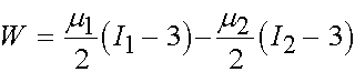
    Of course, any material mechanics, and especially tissue mechanics, can be quite complex, and many assumptions must be made when deriving a consitutitive equation. It is basically impossible to derive a particular constitutive equation that would accurately model all aspects of tissue behavior under any type of loading. This is because tissues may behave very differently under small loads as compared to large loads. For example, under large loads we may expect damage. Also, under different loading rates different tissues may behave differently. Therefore, whenever we develop a constitutive equation to model a tissue, we need to balance the need to accurately model tissue behavior under the range of loading with the need to have a constitutive equation that is simple enough to in a numerical model and to experimentally measure all the constants in the constitutive equation.

    The last issue points to the nature of a constitutive equation. A constitutive equation is typically a phenomenological mathematical model used to describe the relationship between stress and deformation. Although increasingly constitutive models are being developed that relate to morphological aspects of the material, especially for biological tissues, constitutive equations do not describe the microstructural basis for the constitutive behavior. Constitutive equations being phenomenological models, consist of unknown constants, that must be fit with experimental data. Therefore, constitutive equations consist of two major components: constants that must be fit to experimental data and measures of deformation, which may include small or finite deformation as well as the rate of deformation.

    In this section, we will focus on elastic constitutive models for biological tissues. Elastic models are typically the least complex of constitutive equations. However, for tissues within a select range of loading under select conditions, elastic models describe tissue behavior very well. Also, elastic models, including linear elasticity for bone and nonlinear elasticity for soft tissues, have seen wide application in tissue mechanics over the last 30 years.

II. Definition of an Elastic Material

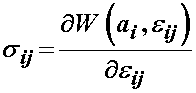
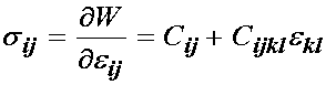
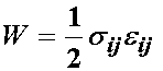
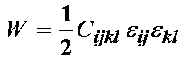
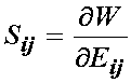
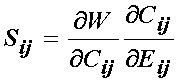
      There are both physical and mathematical defintions of an elastic material. If under applied loads a material stores but does not dissapate energy, and it returns to its orginal shape when the loads are removed, we call that material elastic. This is a physical defintion of an elastic material. If we can define a strain energy or elastic potential function for a material, and when differentiated that strain energy function defines stress in the material, we also call that material elastic. This last defintion can be attributed to George Green, an English mathematician (1791-1840) who had four years of formal education and was largely self-educated. Thus, a strain energy function is sometimes called a Green-elastic function. We can see that the mathematical defintion of an elastic material is related to the physical definition. The main physical characteristic of a purely elastic material is that it stores energy under load. This energy, a scalar quantity, is often called strain energy. Mathematically, an elastic material is one for which a strain energy function can be defined. The scalar strain energy function is usually defined using a W. The strain energy function depends both on a measure of deformation and on constants that must be experimentally determined. Thus, we can write a general relationship between 2nd PK stress and finite strain using a strain energy function as:

                     

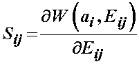
If the tissue undergoes small deformation, then the relationship reduces to that of the Cauchy stress tensor and small strain tensor:

                      

In the next sections, we will discuss more specific forms of strain energy functions and there relevance for tissue characterization.

III. Linear Elastic Constitutive Equations

      The simplest constitutive equation for a solid material or tissue is the linear elastic constitutive equation. This constitutive equation assumes that there is a linear relationship between stress and strain, and that the stress depends only on the strain, not the strain rate. The use of linear elastic constitutive equations is typically restricted for use with bone tissue, since bone tissue is the only tissue that consistently operates in the small strain regime and exhibits a linear relationship between stress and strain. Furthermore, as we discussed in the opening on constitutive equations, the linear elastic assumption is only valid for a select portion of the loading regime of bone. If bone is subject to very rapid loads that would elicit a viscoelastic response, or very large loads that would cause damage or fracture, linear elasticity would not be a valid assumption. However, despite these limitations, linear elastic modeling has proven extremely useful for characterising the mechanical behaviour of bone in a variety of applications. Here we will derive the general linear elastic consitutive equations based on the idea of a strain energy function.

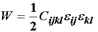
     To begin, we postulate a general quadratic expansion of the scalar energy in terms of the small strain tensor e:

                       

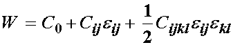
where W is the scalar strain energy, e is the small strain tensor, and the scalar C0, 2nd order tensor Cij and fourth order tensor Cijkl all represent constants to be experimentally determined. Note again that the strain energy function depends on the entities that make up all constitutive equations, including a measure of deformation (the small strain tensor), and constants that have to be determined experimentally. At this point we can begin to make arguments that will simplify the number of constants. First, we recognize that the material will not store any energy if it is not deformed. Therefore, if e is 0, we expect that W should also be zero:

                      

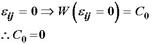
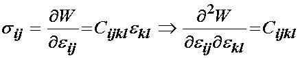
This leads us to the conclusion that C0 must be zero. Next, we differentiate W with respect to the small tensor to obtain the Cauchy stress, as we state in the overview of elasticity:

                   

Again, let us assume the strain is zero. This will give us:

                   

If the strain is zero, we can reasonably expect that the stress in the body should also be zero. Thus, we can conclude that the constants Cij should be zero:

                    

We are thus left with the familiar Hooke's law relationship between stress and strain for a linear elastic material:

                    

As written, there are 81 experimental constants for Cijkl (remember, dimension raised to the power of the number of independent indices, 3^4 = 81). That is a lot of experimental work! Also, we now have the following expression for strain energy in a linear elastic material:

                    

since the Cauchy stress was defined using Hooke's law, we can write the strain energy also as:

                    

At this point, looking at 81 constants (for the 3D case) is pretty intimidating. However, there is hope! We can actually reduce the number of constants by making arguments of symmetry. Let us simplify things a little and look at the 2D case, where there are only 16 constants. This is feasible to write explicitly as:

                 

                   

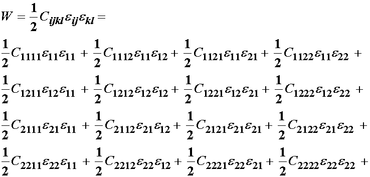
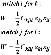
To begin, let us consider the s11 stress. We can then use the symmetry of the strain tensor to switch e12 and e21, subtract the results to get:

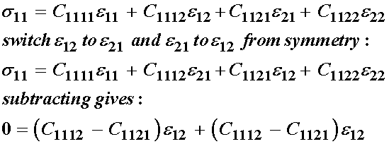
This shows that C1112 equals C1121, reducing the number constants by 1. We perform the same procedure for the rest of the stress components.

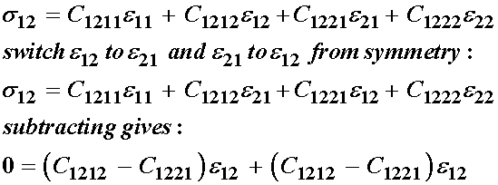
s12:

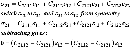
s21:

s22:

                    

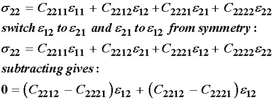
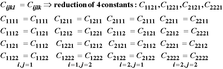
As a result of the strain symmetry, we see that the following constants are equal:

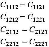
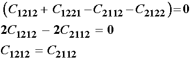
Thus, we have reduced the total number of independent elastic constants by 4 from 16 to 12 due to strain symmetry. Next, let us consider stress symmetry and its affect on the elastic constituents. We recall that s12 = s21, which we write as:

   

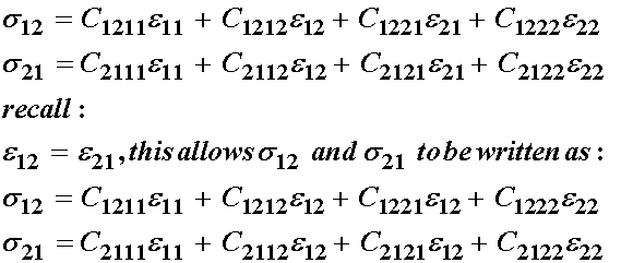
Now we can substract s12 from s21, we will get zero since they are equal:

   

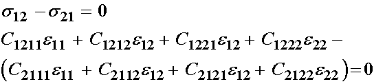
If we group terms by strain we have:

  

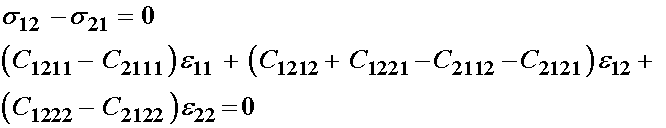
Given that strains are arbitrary and non-zero, for the above equation to hold the quantities in the brackets must be identically zero. Therefore, we see the following equivalence right off and are down to 10 independent constants:

   

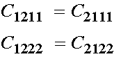
Now let us examine the terms in brackets associates with e12. If we subtitute known equivalences, we have

    

  leaving us with nine independent constants. Likewise, if we make other equivalences:

      

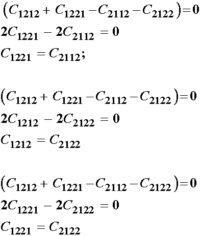
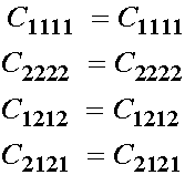
So, finally, after these equivlances, we are down to 6 independent constants of the original 16. If we summarize, we know that do to strain symmetry, we have the following symmetry in elastic constants:

      

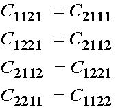
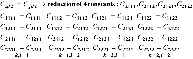
Each switch of kl to lk reduces the number of constants by 1. Since this is done for each cycle of the ij indices, the total reduction in independent constants is 4. Due to stress symmetry, we can write:

       

Again, this symmetry leads to a reduction in the number of independent constants by 4. Finally, consider the expression for strain energy:

        

In this expression, which corresponds to a scalar, all the indices i,j,k,l are dummy indices since they are repeated. Thus, we may rearrange these indices without changing the value of the expression. Let us switch the i and k indices, and then the j and l indices. This gives:

       

since the last terms are also quadratic in strain, we may equate the expressions for energy to get:

       

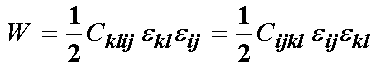
Since both factors are multiplied by the quadratic product of the strain, we may directly equate them as:

        

For the above case, if i = k and j = l, then the above relationship reduces to the trivial case, ie

       

If we have i not equal to k, and j not equal to l, we have:

        

Since two of these are the same, we have a reduction of three elastic constants. So let us summarize the reduction in elastic constants.

1. From Strain Symmetry, we have:

         

2. From Stress Symmetry, we have:

          

we see a further reduction of 4 elastic constants, however, there is an overlap of one constant, so we have actually a reduction of 7 constants.

3. From symmetry of strain energy:

          

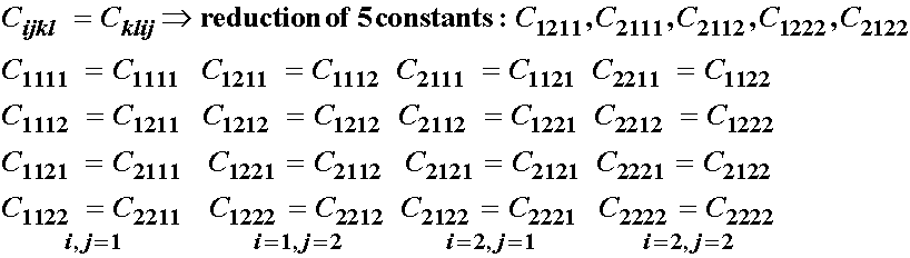
we see a further reduction of 5 elastic constants, however, there is an overlap of 2 constants, leaving a total of 10 reduced constants. Therefore, again, we are only left with 6 independent constants for 2D.

For 3D, we can apply the same analysis. If we consider symmetry of strain, we get a reduction of three constants for

for each index i and j which gives us a reduction of 9*3 = 27, leaving 54 independent constants.. Next, we have symmetry of stress which gives:

In this case we have again 27 potential constants that are reduced, since there are three duplicate ij constants for nine kl constants. However, there is an overlap with C3131, C3232, C2121,C3113, C3223,C2112,C1331,C2332,C1221, leaving us to reduce the number of independent constants by 18. This leaves us with 36 independent constants.

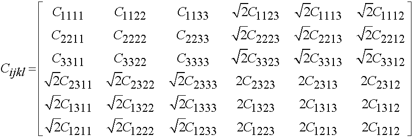
Again, we have major symmetry due to the existence of a strain energy function. This allows us to reduce the number of indpendent constants by 15 to 21. Thus, for any linear elastic material we need to measure at most 21 constants.     

Thus, we can write the general form of the linear elastic constitutive matrix as:

   

However, in real life even these 21 independent constants are simplifed to 2, 5, or 9 depending on material symmetry.

If there are 9 independent constants, then the material is orthotropic, and has the form:

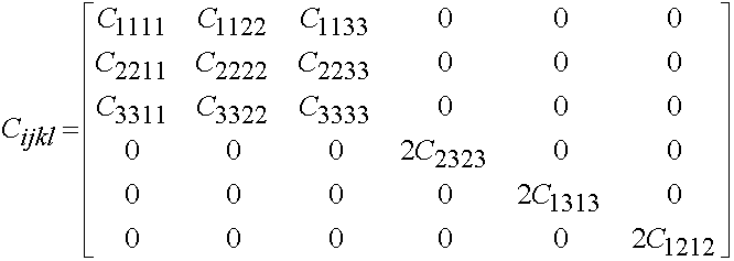
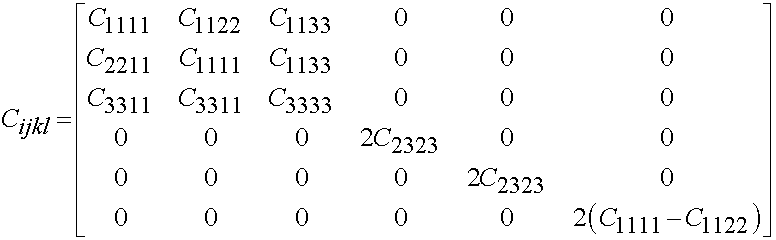
If there are 5 independent constants, then the material is transversely isotropic and has the form

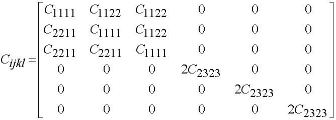
Finally, if there are 2 independent constants, then the material is isotropic and has the form:      

We will see in the section on bone mechanics that the above linear elastic constitutive matrices may be related to the hierarhical bone structure in structure-function relationships.

III. Non-Linear Elastic Constitutive Equations

      From a specific strain energy function, we could derive the linear elastic coefficients by differentiating the strain energy with respect to the small strain coefficients. We could dervie both isotropic and anisotropic elastic coefficients from the strain energy function. However, in the linear elastic case, we have a linear proportion between the Cauchy stress tensor and the small deformation strain tensor. Since we were operating in the realm of small deformation mechanics, then the Cauchy stress tensor is equivalent to the other stress tensors. Furthermore, since we assumed a linear relationship between stress and strain. we have a unique and defined relationship between stress and strain completely embodied in the elastic constants fo Hooke's law. While linear elasticity is a very good model for bone tissue, it does not serve very well for soft tissue mechanics for two reasons. First, most soft tissues undergo strains that qualify as large deformation. Second, the relationship between stress and strain for soft tissues is generally nonlinear. This means that the stiffness of a soft tissue will change with deformation, unlike a linear elastic model where the stiffness is constant as long as the material is in the elastic range.

   In this section, we will cover the many aspects of strain energy functions for nonlinear elastic materials. It is important to note that unlike for linear elastic materials, there is no "one" material model for a nonlinear elastic material. There are many potential strain energy functions, and indeed for soft tissues we will encounter a plethora of strain energy functions for each different type of tissue.

III. A General Considerations for Nonlinear Elastic Strain Energy Functions

    To begin with, we write the general expression for stress in terms of the strain energy function. If we consider a general nonlinear material that can undergo finite deformation, then we need to write the strain energy as a function of the deformation gradient tensor or the finite strain tensor. Recall that a constitutive equation depends on a deformation measure and constants to be determined experimentally. Thus, in the most general form we can write that the strain energy function depends on the deformation gradient tensor or the finite strain tensor. If the strain energy function W depends on the deformation gradient, we obtain the 1st PK stress when we differentiate the strain energy function with respect to the deformation gradient tensor:

  

If we differentiate the strain energy function depending on the finite strain tensor with respect to the finite strain tensor, we obtain the 2nd PK stress tensor

:

These are the most generalized forms of strain energy functions and the resulting stress tensors they generate. We have some further restrictions on the strain energy function that apply to all materials. First, we understand that if there is no deformation, than no energy should be stored in the material. This would amount to the deformation gradient being equal to the identity tensor, or the finite strain tensor being zero. Thus, we have:

Likewise, we need to restrict the strain energy function such that is is positive (energy must be by definition positive) for any deformation:

Finally, we need a physical restriction such that we cannot infinitely expand a material or crush it such that it has zero volume. In both of these cases, we would require infinite strain energy, something that is not physically possible. Thus, we write:

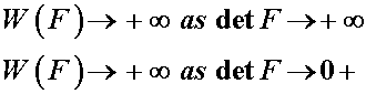
Thus, these are general restrictions on the strain energy function. Note that these would also apply in the case of small deformation elasticity.

The final requirement we place on the strain energy function is that it does NOT depend on any rigid body motion, that is on translation or rotation. Let us assume that there is an initial deformation denoted by the deformation gradient tensor F. Next, let us apply a further rigid body motion. This will create a new deformation gradient tensor F*. Since we know that the energy won't change under a rigid body motion, then the energy under F and F* must be equivalent:

Furthermore, we know that pure translation won't change F. Let us consider that F* is a rotation of the original deformation state F embodied in the rotation tensor R. Then we have:

However, recall that we can write any deformation gradient tensor into a rotation times a stretch component. Thus, we can write the right hand side as:

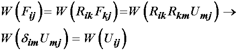
This result shows that the strain energy function depends only the stretch (deformation) portion of the deformation gradient tensor, not on the rotation component. Since both the right Cauchy deformation tensor and the finite strain tensor can be written in terms of the right stretch tensor:

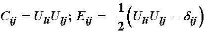
Then it follows that the strain energy tensor may also be written in terms of the right Cauchy deformation tensor and the finite strain tensor:

The above indicates that a strain energy function for a general nonlinear elastic material can be written in terms of a deformation gradient tensor, a right Cauchy deformation tensor, or the finite strain tensor.

We know that the differentation of the strain energy function with respect to the finite strain tensor will give the 2nd PK stress tensor.

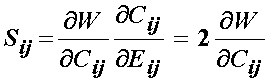
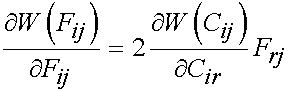
The question then becomes how we need to differentiate the strain energy function with respect to the right Cauchy deformation tensor. To do this we simply apply the chain rule to the above differentiation to give:

Recall that we can write the finite strain tensor in terms of the right Cauchy deformation tensor as:

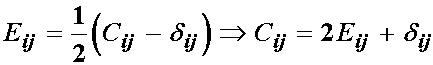
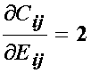
This means that when we differentiate the right Cauchy deformation tensor with respect to the finite strain tensor the result is simply 2:

This means that the 2nd PK stress may be calculated directly from a strain energy function written in terms of the right Cauchy deformation tensor as:

III. B General Isotropic Hyperelastic Materials

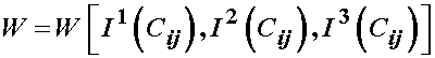
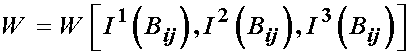
    The most basic constitutive equation for a hyperelastic material is that derived from an isotropic strain energy function. Based on the representation theorem for invariants, a fundamental result for a scalar-valued function of tensors that is invariant under rotation (that is, it is isotropic) is that this function may be expressed in terms of the principal invariants of its argument. Since the arguments for the strain energy function are F, C, or E, that are second order tensors with three invariants, it follows that an isotropic hyperelastic material can be defined in terms of three invariants as the deformation measures. Thus, we can write a general strain energy function as:

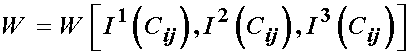
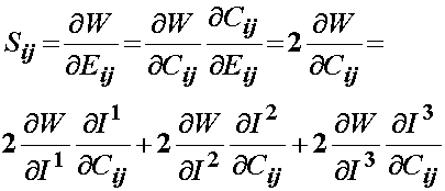
where I1, I2, and I3 denote the three invariants of C. Based on the above representation, we can again use the chain rule to write the 2nd PK stress as:

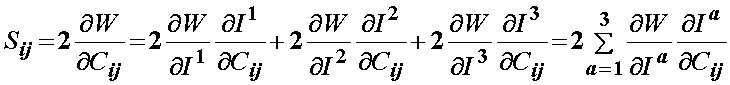
We can see from the above that the dependence of W on the invariants will vary for differ proposed constutive models. However, the dependence of the right Cauchy deformation tensor on the invariants I will be the same no matter what the constitutive models. Let us now consider each invarieant in term.

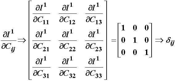
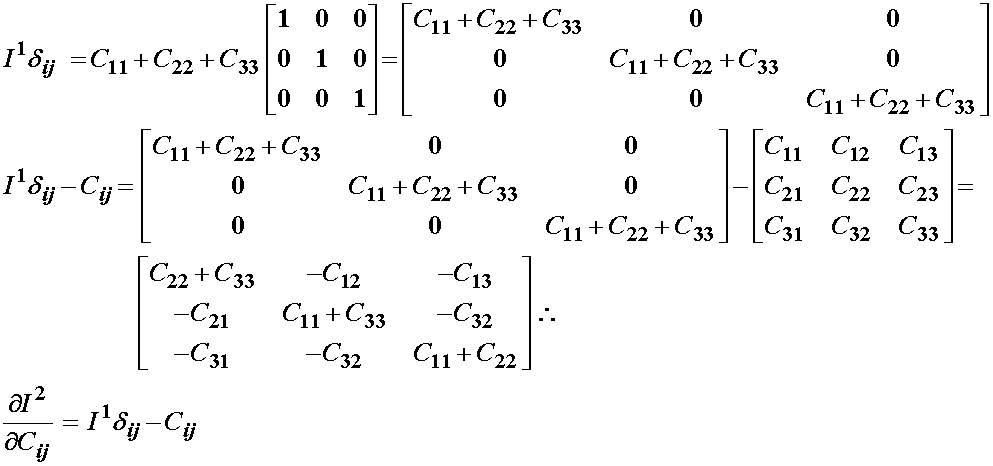
The first invariant of the right Cauchy deformation tensor, as for any 2nd order tensor is:

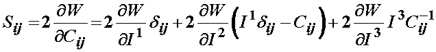
If we differentiate the scalar I1 with respect to every element of the right Cauchy deformation tensor, we obtain a second order tensor back, namely the Kronecker delta or identity tensor:

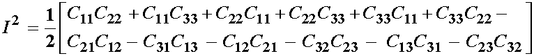
We define the second invariant for a 2nd order tensor as:

We again differentiate the above invariant with respect to all elements of the right Cauchy deformation tensor to obtain:

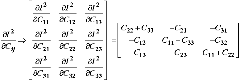
Since we have shown C to be symmetric, we can rewrite the above as:

Although not readily apparent, if we multiply the first invariant by the identity and substract the original right Cauchy deformation tensor from this quantity, we obtain the derviative of the second invariant with respect to the right Cauchy deformation tensor:

 

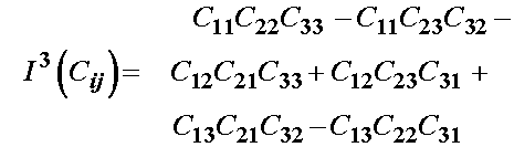
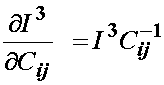
Now let us consider the differentiation of the third invariant of C. From the section on invariants in the mathematical preliminary section, this may be written as:

We then differentiate the third invariant with respect to C to obtain:

  

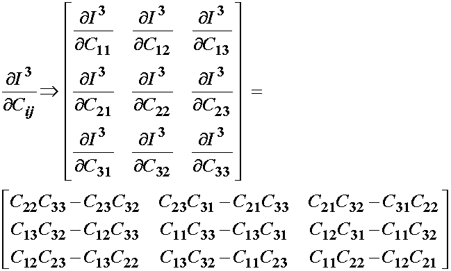
While it is not readily apparent, we can write the above definition of the third invariant using the MATLAB symbolic manipulator. First, we take the inverse of the right Cauchy deformation tensor. This is first done by making symbols of the right Cauchy Deformation tensor C, making a matrix of C, and then taking the inverse using the inv command:

>> syms c11 c12 c13 c21 c22 c23 c13 c23 c33
>> c = [c11 c12 c13; c21 c22 c23; c13 c23 c33]

c =

[ c11, c12, c13]
[ c21, c22, c23]
[ c13, c23, c33]


>> cinv = inv(c)

cinv =

[ (c22*c33-c23^2)/(c11*c22*c33-c11*c23^2-c21*c12*c33+c21*c13*c23+c13*c12*c23-c13^2*c22), -(c12*c33-c13*c23)/(c11*c22*c33-c11*c23^2-c21*c12*c33+c21*c13*c23+c13*c12*c23-c13^2*c22), (c12*c23-c13*c22)/(c11*c22*c33-c11*c23^2-c21*c12*c33+c21*c13*c23+c13*c12*c23-c13^2*c22)]
[ (-c21*c33+c13*c23)/(c11*c22*c33-c11*c23^2-c21*c12*c33+c21*c13*c23+c13*c12*c23-c13^2*c22), (c11*c33-c13^2)/(c11*c22*c33-c11*c23^2-c21*c12*c33+c21*c13*c23+c13*c12*c23-c13^2*c22), -(c11*c23-c13*c21)/(c11*c22*c33-c11*c23^2-c21*c12*c33+c21*c13*c23+c13*c12*c23-c13^2*c22)]
[ -(-c21*c23+c13*c22)/(c11*c22*c33-c11*c23^2-c21*c12*c33+c21*c13*c23+c13*c12*c23-c13^2*c22), -(c11*c23-c12*c13)/(c11*c22*c33-c11*c23^2-c21*c12*c33+c21*c13*c23+c13*c12*c23-c13^2*c22), (c11*c22-c12*c21)/(c11*c22*c33-c11*c23^2-c21*c12*c33+c21*c13*c23+c13*c12*c23-c13^2*c22)]

From the above, although it may be difficult to see, there is a common denominator for all the terms in the inverse, it is:

(c11*c22*c33-c11*c23^2-c21*c12*c33+c21*c13*c23+c13*c12*c23-c13^2*c22)

However, we can recognize this as the determinant of C if we take the determinant in MATLAB:

>> cdet = det(c)

cdet =

c11*c22*c33-c11*c23^2-c21*c12*c33+c21*c13*c23+c13*c12*c23-c13^2*c22

If we then multiply the Inverse of C times the determinat of C in MATLAB we obtain:

>> cdet*cinv

ans =

[ c22*c33-c23^2, -c12*c33+c13*c23, c12*c23-c13*c22]
[ -c21*c33+c13*c23, c11*c33-c13^2, -c11*c23+c13*c21]
[ c21*c23-c13*c22, -c11*c23+c12*c13, c11*c22-c12*c21]

which, if we account for the symmetry of C, is equivalent to the derivative of I3 with respect to C. Thus, we can write the derivative of I3 with respect to C, recognizing that the det of C is the third invariant, we can write:

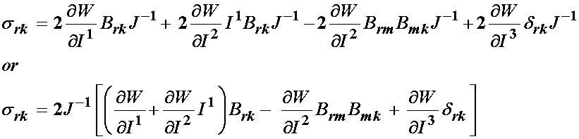
Thus, for the most general isotropic form of the nonlinear elastic strain energy function we have:

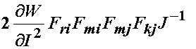
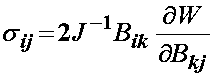
We obtain the 2nd Piola-Kirchoff stress from this strain energy function by differentiating the strain energy function with respect to C, using the chain rule:

Using the expressions for the derivatives of I1, I2, and I3 dervied above, we can write the 2nd PK stress for an isotropic strain energy function written in terms of invariants of the right Cauchy deformation tensor as:

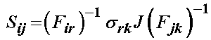
To obtain the Cauchy stress tensor from the above relation, we recall the relationship between the Cauchy and 2nd PK stress tensors derived in the section on alternative stress tensors:

Substituting into the above relationship, we obtain:

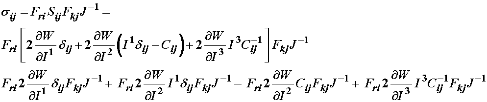
We can simplify the above expression by looking at specfici terms. First consider the terms:

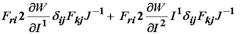
In these sets of terms we have the common term:

which we can rewrite using the Kronecker delta as:

We can recognize the above term from the strain deformation section as the left Cauchy Deformtion tensor:

Thus, the first two terms of the Cauchy stress tensor for an isotropic strain energy function may be written as:

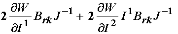
Let us now consider the last two terms:

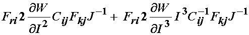
If we examine the first term, we recall that we can write the right Cauchy deformation tensor as:

Thus, for the first term we have, noting that k in the above expression is a dummy index which we replace with m:

We note that the product of F's above give the left Cauchy deformation tensor, leaving us:

Turning our attention to the last term, we break down the inverse of C into its components to give:

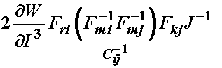
The two F and inverse F terms will produce the Kroneker delta, giving:

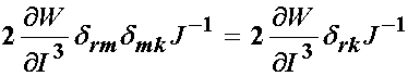
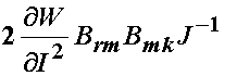
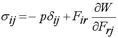
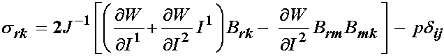
Thus, we can write the simplified form of the Cauchy stress tensor for an isotropic nonlinear hyperelastic material as:

Of course, there are other deformation measures in terms of which we can write W, namely the left Cauchy deformation tensor and the principal stretch ratios. If we write the isotropic strain energy function in terms of the left Cauchy deformation tensor, we have:

Without proof (see Holzapfel, 2000), we can write the Cauchy stress tensor in terms of a strain energy function using the left Cauchy deformation tensor as:

To see the equivalent 2nd PK stress, we use the transformation between the 2nd PK stress and the Cauchy stress tensor:

Substituting in for the Cauchy stress tensor above, we obtain:

Next, we recall that the left Cauchy deformation tensor is written in terms of the deformation gradient tensor. This allows us to write the above as:

Finally, many nonlinear elastic models write the strain energy function in terms of principal stretches:

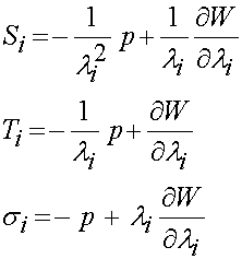
Then we can write the 2nd PK stress, the 1st PK stress, and the Cauchy stress as:

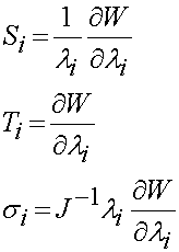
where only one index is used for the stress tensor since the derivative of W with respect to the principal stretch tensors gives the prinicpal stresses, of which there are three.

 

 

III.C Incompressible Isotropic Hyperelastic Materials

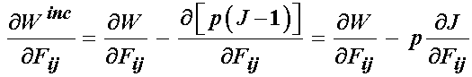
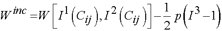
    Many soft tissues are characterized as incompressible. This means that the volume of the tissue will not change during deformation, no matter how high the hydrostatic pressure. If we recall that the Jacobian J, the determinant of F is the ratio of the volume in the deformed configuration to the volume in the reference configuration, then the constraint that no volume change occur is equivalent to the constraint that J = 1. If we assume in compressibility, this means that the hydrostatic pressure is no longer determined by the strain energy function, and that we have to add the incompressibility condition as a constraint on the strain energy function. If we write the strain energy function dependent on the deformation gradient F, then we can write the general strain energy function modified for incompressibility as:

    

where p is now a Lagrange multiplier, similar to that we saw in the section on optimization. The associated constraint with the Lagrange multiplier is the incompressiblility condition, J - 1. In fact the Lagrange multiplier p has a physical meaning, namely it is the hydrostatic pressure. We can derive the 1st PK stress by diferentiating the above strain energy function with respect to F. One of the more tedious terms to differentiate is the determinant of F or J with respect to F. To do this, we again turn to the MATLAB symbolic tookbox. We first generate the symbols of F, then take the determinant:

>> syms f11 f12 f13 f21 f22 f23 f31 f32 f33
>> f = [f11 f12 f13; f21 f22 f23; f31 f32 f33]

f =

[ f11, f12, f13]
[ f21, f22, f23]
[ f31, f32, f33]


>> fdet = det(f)

fdet =

f11*f22*f33-f11*f23*f32-f21*f12*f33+f21*f13*f32+f31*f12*f23-f31*f13*f22

Next, since we are differentiating the determinant of F or det(F) = J, with respect to F, we are differentiating a scalar with respect to a second order tensor, we will obtain a second order tensor. We can do this in the MATLAB symbolic toolkit as:

>> jacobian(fdet,f)

ans =

[ f22*f33-f23*f32, -f12*f33+f13*f32, f12*f23-f13*f22, -f21*f33+f31*f23, f11*f33-f31*f13, -f11*f23+f21*f13, f21*f32-f31*f22, -f11*f32+f31*f12, f11*f22-f21*f12]

We use the "Jacobian" function in MATLAB, as this allows differentiation of a scalar or vector directly with respect to a vector or matrix. Doing this gives the following result:

>> jacobian(fdet,f)

ans =

[ f22*f33-f23*f32, -f12*f33+f13*f32, f12*f23-f13*f22, -f21*f33+f31*f23, f11*f33-f31*f13, -f11*f23+f21*f13, f21*f32-f31*f22, -f11*f32+f31*f12, f11*f22-f21*f12]

Although not readily clear, we can acutally write that the derivative of the Jacobian with respect to F is equal to J multiplied by F inverse transpose. First, let us take the inverse of the transpose of F using the symbolic toolkit:

>> ftinv = inv(transpose(f))

ftinv =

[ (f22*f33-f23*f32)/(f11*f22*f33-f11*f23*f32-f21*f12*f33+f21*f13*f32+f31*f12*f23-f31*f13*f22), -(f21*f33-f31*f23)/(f11*f22*f33-f11*f23*f32-f21*f12*f33+f21*f13*f32+f31*f12*f23-f31*f13*f22), (f21*f32-f31*f22)/(f11*f22*f33-f11*f23*f32-f21*f12*f33+f21*f13*f32+f31*f12*f23-f31*f13*f22)]
[ -(f12*f33-f13*f32)/(f11*f22*f33-f11*f23*f32-f21*f12*f33+f21*f13*f32+f31*f12*f23-f31*f13*f22), (f11*f33-f31*f13)/(f11*f22*f33-f11*f23*f32-f21*f12*f33+f21*f13*f32+f31*f12*f23-f31*f13*f22), -(f11*f32-f31*f12)/(f11*f22*f33-f11*f23*f32-f21*f12*f33+f21*f13*f32+f31*f12*f23-f31*f13*f22)]
[ (f12*f23-f13*f22)/(f11*f22*f33-f11*f23*f32-f21*f12*f33+f21*f13*f32+f31*f12*f23-f31*f13*f22), -(f11*f23-f21*f13)/(f11*f22*f33-f11*f23*f32-f21*f12*f33+f21*f13*f32+f31*f12*f23-f31*f13*f22), (f11*f22-f21*f12)/(f11*f22*f33-f11*f23*f32-f21*f12*f33+f21*f13*f32+f31*f12*f23-f31*f13*f22)]

We next multiply this by J to obtain:

>> ftinv*fdet

ans =

[ f22*f33-f23*f32, -f21*f33+f31*f23, f21*f32-f31*f22]
[ -f12*f33+f13*f32, f11*f33-f31*f13, -f11*f32+f31*f12]
[ f12*f23-f13*f22, -f11*f23+f21*f13, f11*f22-f21*f12]

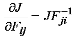
This is the same as the derivative of J with respect to F. Thus, we can write:

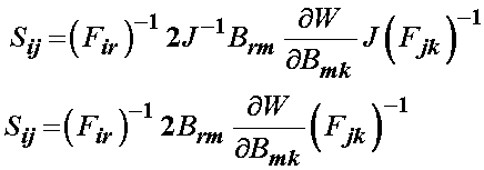
We write the general derivative of W with respect to F:

If we substitute for the derivative of J with respect to F, we obtain:

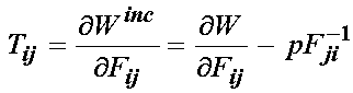
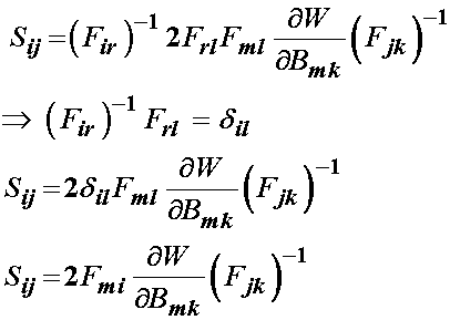
If we wish to generate the 2nd PK stress for an incompressible stress is obtained by muliplying the 1st PK stress by the inverse of the deformation gradient:

If we apply the transformation of the 2nd PK stress and 1st PK stress to the incompressible form of the 1st PK stress we obtain:

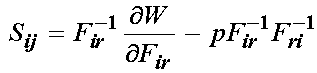
One property that we state without proof for strain energy functions is the following:

Thus, given that F inverse times F inverse gives C inverse, and the relationship above, we can write the 2nd PK stress for an incompressible nonlinear elastic material as:

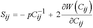
Finally, we can write the Cauchy stress for a general incompressible hyperelastic material as:

If we define the strain energy function in terms of three invariants for an isotropic incompressible material, we write the strain energy function as:

where I3 as the third invariant is equal to one since there is no volume change, and p is again the hydrostatic pressure.

To compute the 2nd PK stress we again take the derivative of W with respect to C. It is very similar to the original isotropic 2nd PK stress from a strain energy function, except there is no dependence on I3:

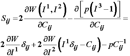
where again we have used the fact that the derivative of the third invariant or determinant of a tensor with respect to the tensor itself gives the inverse of the original tensor in taking the derivative of the term associated with the hydrostatic pressure. We can similarly get the Cauchy stress for an incompressible isotropic material with a modification of the strain energy function for the hydrostatic pressure as:

Finally, we can express the Cauchy, 1st PK and 2nd PK stresses in for an incompressible material as:

which has similarities to these stresses without the incompressibility constraint.

III.D   Specific Forms of Isotropic Strain Energy Functions

Up to now, we have presented general forms of strain energy functions for isotropic hyperelastic materials. However, to actually define a constitutive model we need to have a specific form of a strain energy function. In this section, we present a few specific strain energy functions that have been proposed for isotropic hyperelastic materials. Most of these strain energy functions have found applications for analyzing rubber and polymers.

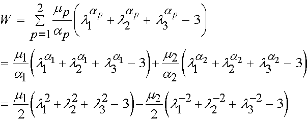
One general strain energy function that has found significant use is that due to Ogden. The Ogden strain energy function is written in terms of the principal stretches as:

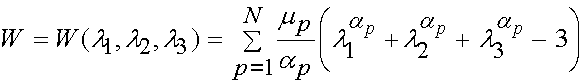
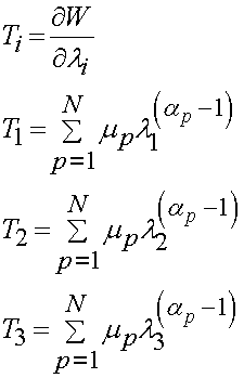
where l1,l2, and l3 are the principal stretch ratios and mp and ap are constants to be determined experimentally for every value of p. Note that p can run from 1 to N terms. Also, it is important to reemphasis that this strain energy function contains the two components we need in all strain energy functions, namely a measure of deformation (the principal stretch) and constants that are determined experimentally. If we apply the equations for deriving the Cauchy, 1st PK and the 2nd PK stress from a strain energy function derived in terms of principal stretches, we can either differentiate the strain energy function analytically or in MATLAB. If we do this analytically for the 2nd PK stress we obtain:

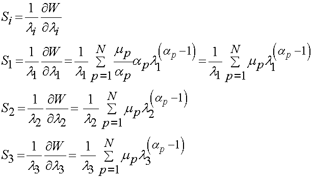
were again S1, S2 and S3 are the principal 2nd PK stress. For the principal Cauchy stress we have:

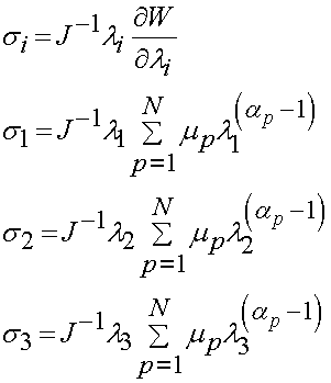
and finally for the principal 1st PK stress we have:

Two classic forms of the strain energy function may be derived from the Ogden model and are known as the Mooney-Rivlin model and the neo-Hookian model. These models are been generally applied to analyze rubber and assume incompressibility. Incompressibility for deformation defined in terms of prinicpal stretch is easy to calculate since the volume ratio is defined as:

For the Mooney-Rivlin model, we use N = 2, a1 = 2 and a2 = -2 in the Ogden model. This gives us:

Now, let us consider how these may be defined in terms of the invariants. Recall that the right Cauchy deformation tensor is defined in terms of the stretch tensor U as:

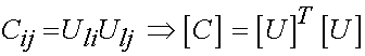
The principal stretches are the eigenvalues of U, so U may be written in terms of the principal stretches as:

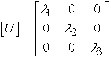
Thus, we define C in terms of principal stretches as:

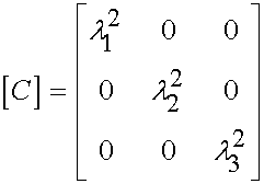
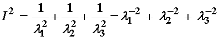
The first invariant of C is the trace of C (sum of the diagonal terms), so this gives:

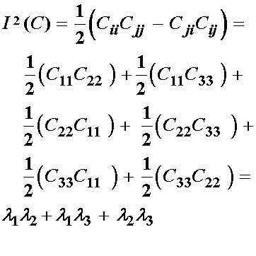
Now let us conside the second invariant of C. If we follow the index representation of the second invariant we have:

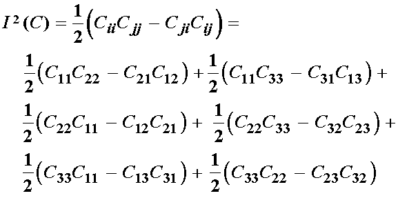
which in the case of principal stretch reduces to:

However, recall the incompressibility constraint. In this case we can substitute for l3 with the following:

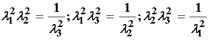
If we substitute the above relationship obtained from the incompressibility constraint into the 2nd Invariant from the principal stretches, we obtain:

The above relationship for the second invariant derived using the incompressibility constraint is equivalent to the second term in the Mooney-Rivlin strain energy function. Thus, we can write the final form of the Mooney-Rivlin strain energy function as:

The neo-Hookian strain energy function is obtained from the Ogden strain energy function by setting N = 1, a1 = 2. This gives us:

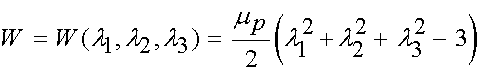
Since we have already established that the first three terms in the parentheses constitute the first invariant of the right Cauchy deformation tensor, we have the neo-Hookian strain energy function written as:

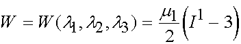
Another model for isotropic hyperelasticity is the Varga model. It is obtained by setting N = 1 and a1 = 1 in the Ogden model:

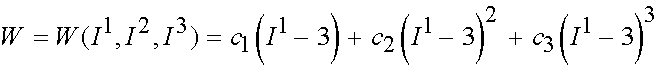
The above isotropic strain energy functions could be derived as special cases of the Ogden strain energy function. There are other widely used strain energy functions that are not derived from the Ogden strain energy function. We detail these strain energy functions next. The first of these is the Yeoh strain energy function. It is written as:

The second is the Arruda and Boyce strain energy function, that was dervied based on statisical models of chain orientations in polymers. The first three terms are written as:

where m denotes the shear modulus and n is the number of segments in a chain jointed at chemical crosslinks.

The last specific strain energy function we will present for isotropic materials is that of the Blatz-Ko model. The model was formulated for elastomeric foams which are compressible. Thus, unlike the specific forms of the strain energy functions presented previously, the Blatz-Ko model is for compressible materials. This model is written as:

III E Transversely Isotropic Strain Energy Functions

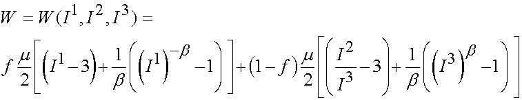
  Most isotropic strain energy functions were developed for rubber materials and polymers. Because of the random nature of the microstructure, the isotropic strain energy functions fit this material behavior well. Although these strain energy functions have been adopted to biological tissues, in some cases fitting data very well, many biological tissues are not isotropic, due to perferred orientations in the microstructure. Thus, we have to look to anisotropic strain energy functions to characterize these tissues. In general, anisotropic strain energy functions based on invariants assume some type of embedded fiber. This corresponds with many biologic soft tissues, that have for example collagen fibers embedded in them.

To start with, we are interested in how much the embedded fibers within a matrix stretch. If we consider a unit vector a0, then the vector in the deformed configuation that results from a0 is obtained using the deformation gradient tensor Fij as:

However, since a0 is a unit vector, then a as a vector really represents how much a0 has been stretched during deformation. Thus, if we take the square of the length of a, this will give the square of the stretch ratio l, as:

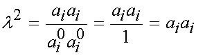
However, if we substitute for a with the deformation gradient times a0, we obtain:

The center F terms are simply the right Cauchy deformation tensor, so we have:

This shows that the fiber stretch depends on the initial fiber direction a0 and the right Cauchy deformation tensor C.

If we assume that the strain energy function is transversely isotropic, then the strain energy function (which is also referred to as the Helmholtz free-energy function) should depend on both the right Cauchy deformation tensor and the fiber orientation. We can therefore write the transversely isotropic strain energy function formally as:

were the dyadic product of the initial fiber direction vector creates a second order tensor having the same tensorial order as the right Cauchy deformation tensor.

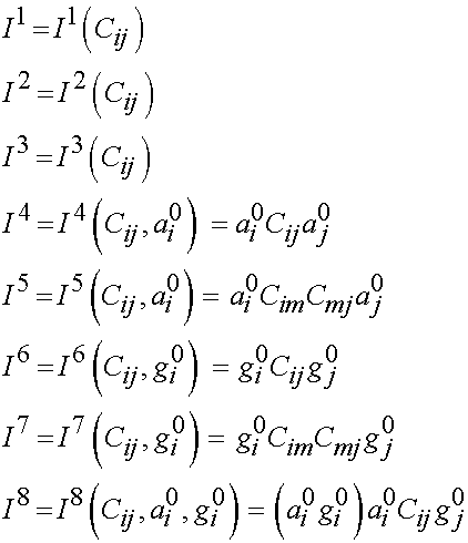
Just as a transversely isotropic linear elastic material has more constants than an isotropic linear elastic material, so does a transversely isotropic strain energy function depend on more invariants than an isotropic strain energy function. In fact, the transversely isotropic strain energy function actually depends on five invariants. The first three invariants are the 1st, 2nd and 3rd invariants of the right Cauchy deformation tensor. The fourth and fifth invariants depend on both the right Cauchy deformation tensor and the initial fiber direction vector. The 4th and 5th invariants describe the anisotropy arising from a preferred fiber direction.

These 4th invariant is written as:

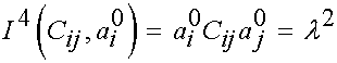
note that this invariant actually represents the stretch of the initial fibril direction vector.

The 5th invariant is written as:

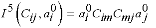
With five invariants, we write the general transversely isotropic strain energy function as:

Similar to the isotropic strain energy function, we can derive the 2nd Piola-Kirchoff stress tensor from the transversely isotropic strain energy function by taking the derviative of the strain energy function with respect to C, only this time we have to sum the derivative for five invariants:

The first three terms of the 2nd Piola-Kirchoff stress is the same as for the isotropic strain energy function. The last two terms we derive as:

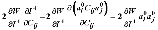
and

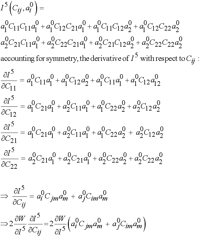
Thus, by combining the derivatives of the first three invariants from the isotropic strain energy function with the dervivative of the 4th and 5th invariants from the second strain energy function, we obtain the 2nd PK stress from a transversely isotropic strain energy function:

:

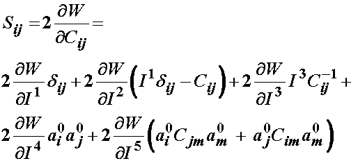The derivative of W with respect to I4 represents the contribution of the fibers, while the derivative with respect to I5 represents the interaction of the fiber and the matrix.

III F Orthotropic Strain Energy Functions

  The last class of strain energy functions we will consider is the orthotropic strain energy function. This type of strain energy function is especially relevant to matrices with two types of embedded fibers. This occurs in biological tissues for example in arterial walls and the intervertebral disk. In this case, we introduce another direction vector for the second fiber named g0. This direction vector g0 has the same properties as the direction vector a0, namely:

To accomodate the additional degree of anisotropy, we need to use eight invariants. These include the three invariants from the isotropic strain energy function and two invariants from the transversely isotropic strain energy function. In addition, we now have two invariants from the second fiber family (giving 7 invariants) and 1 more invariant that accounts for the interaction in deformation between the fiber families (giving a total of 8 invariants). These invariants are:

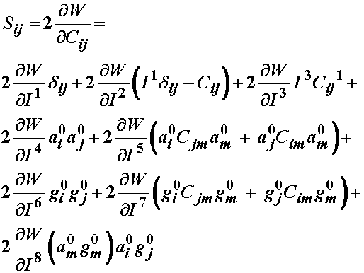
Again, we may expand the expression for the 2nd PK stress from the transversely isotropic strain energy function to obtain the following expression for 2nd PK stress from an orthotropic strain energy function:

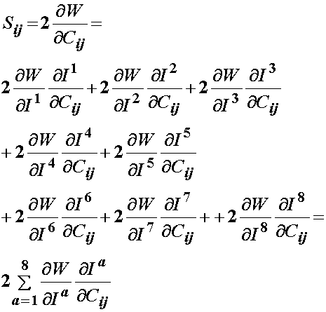
The derivatives for the first five invariants have already been developed. The derivatives for the 6th and 7th invariants with respect to the right Cauchy deformation tensor C are the same as the 4th and 5th invariant derivative, respectively, with a0 being replaced by g0:

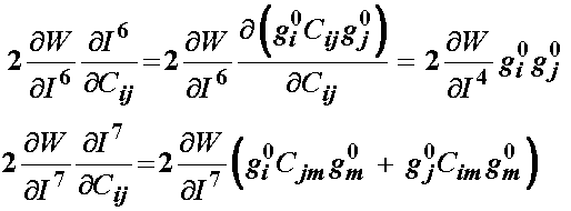
This leaves us to determine the derivative of C with respect to the 8th and last invariant, which represents the interaction between the two fiber families. We note that the first term is the dot product of a0 and g0 and does not depend on C. We note that the second term is similar to both the 4th and 6th invariant, with one a being replaced by a g or vice versa. Thus when we take the derivative we have:

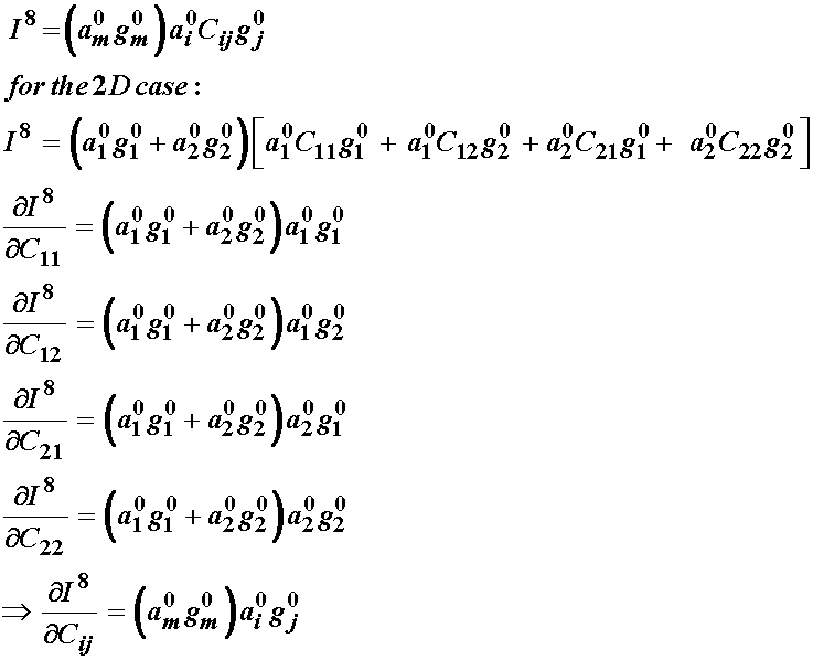
Thus, we have the 2nd PK stress from the general orthotropic strain energy function gives:

 

IV. Relationships between Linear and Non-linear Elasticity

      A question that arises is whether there is a relationship between linear and non-linear elasticity. One piece of common ground is that we may write a strain energy function for both linear and non-linear elastic materials. The other relationship can be gleaned by considering the following. In both linear and non-linear elasticity, if we differentiate the strain energy function with respect to the strain, we obtain the stress. In the case of small deformation the Cauchy stress, in the case of large deformation the 2nd PK stress. If we take a look at Hooke's law for a linear elastic material, it becomes clear that if we differentiate the strain energy function twice with respect to the strain we obtain the Hooke's law constants:

It is clear for linear elasticity that Cijkl will be constant irregardless of deformation. It turns out that if we differentiate any strain energy function with respect to either the finite strain tensor or the right Cauchy deformation tensor we obtain elastic "constants". However, for the case of a nonlinear material, these elastic "constants" will differ depending on the level of deformation. Mathematically, we take the second derivative of the strain energy function, we are in fact taking the first derivative of the stress-strain curve. Hence, at any point on the stress strain curve we are obtaining the tangent to that curve at any point, i.e. any amount of deformation. Thus, we refer to the elastic "constants" obtained by differentiating the strain energy function twice as the tangent elastic propeties. This procedure is very critical to solving finite element problems for large deformation nonlinear elasticity. For small deformation linear elasticity the tangent elastic constants are equivalent to the overall elastic properties since the stress-strain curve is linear and stiffness therefore does not change as deformation changes. However, for a nonlinear elastic material, the slope of the stress-strain curve changes with deformation, hence the instantaneous stiffness of the material changes with deformation. We will see that this is a quite common occurence with soft tissues, as the generally become stiffer with increased deformation. Thus, we can derive the tangent elastic properties for any material linear or nonlinear as:

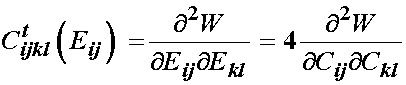
where Cijkl with the small t superscript denotes a tangent elastic coefficient, and may be derived either from the finite strain tensor or the right Cauchy deformation tensor. In the case of a linear material, the tangent properties will not change with strain.

V. Summary

In summary, we have described constitutive models for both linear and non-linear elastic materials. Of course, these are models and as such are idealizations. However, these models are proven quite useful in both hard and soft tissue biomechanics. Furthermore, based on these elastic constitutive models, which do take into account material behavior, we now have nine more equations, those relating stress to strain, that we did not have previously. Thus, we now have completed what we need to solve any solid mechanics problems, namels the same number of equations as unknowns. According to the chart below, we have added nine new equations using a constitutive model to relate stress and strain, but have not added any more unknowns, giving us equal unknowns and equations (21 each, or if we account for symmetry, 15 each):

Equations Type	# of Equations	Unknown Quantity	# Unknowns	Independent Unknowns
Equilibrium	3	stress sij	9	6
Strain Displacement	9	strain eij, displacement ui	12	9
Constitutive	9	No new unknowns	0	0

Thus, we now have all the information we need to solve a biosolid mechanics problem. Of course, we must make assumptions regarding the materials behavior. Still, these constitutive models serve a vital role in biosolid mechanics as they are a quantitative measure of tissue function. We can therefore relate the tissue structure to this function, and derive a structure-function relationship, which can give us a quantitative idea of how alterations in tissue structure due to aging or disease affect its function.