I. Overview

    Now that we have defined constitutive models, the next step is to fit these models to experimental data to define the model constants. After all, it is all well and good to propose a constitutive model, but unless this constitutive model can be fit to a particular tissue behavior, it is not of much use. Furthermore, it is good to keep in mind that constitutive models are phenonenological, and as such seek to characterize material mechanical behavior without knowing in detail the ultrastructural phyics that give rise to such material. Of course, if possible, the constitutive model seeks to utilize such knowledge when choosing the model. Still, the constants of the model are based purely on observation of material response under experimental conditions.

   The critical question then becomse out to fit a particular model. Since constitutive models relate stress and strain, we ideally need to know the stress and strain state. From this stress and strain state we can then backcalculate or fit the constants from the constitutive model. This can be quite straightforward when we are dealing with the simplest constitutive model, isotropic linear elasticity. In this case, we may perform a uniaxial test, measure the longitudinal and transverse deformation, calculate the stress based on the measured load and initial specimen area, and then calculate a Young's modulus and Poisson ratio. However, when the material behavior is nonlinear and/or time dependent, fitting constants for the constitutive model becomes much more invovled. For these cases, we must typically do multiple tests and then try to mathematically fit the constitituve model to the data in some best sense. Note the words "best sense". In mathematics, "best sense" typically means optimization. In optimization, we try to minimize or maximize a quantity, often times with constraints. To fit constitutive data, we are going to try and minimize the square of the difference between the experimental measurement of stress and that calculated by the constitutive model using a numerical algorithm. The algorithm will adjust the constants within the chosen constitutive model to minimize the error. The result gives the constants of the constituent model that best fit the data.

This section describes how to perform the best fit of data, from setting up the minimization problem, to the experimental data required, to performing the numerical calculations in MATLAB. At the end of this section, you should:

1. Understand the concept of the minimization fitting process
2. Understand the experiments required to obtain necessary data
3. Be able to set up and perform the minimization calculation in MATLAB
4. Understand how to evaluate the fit, including necessary physical constraints on the Data

II. Optimization Basics

    The basic concept of optimization is familiar at least intiutively to everyone, and we use it constantly making decisions in our lives. For example, if we are performing a certain task, we probably seek to do this task to attain a certain objective, with a constraint that the task only take so much time. Or, we may choose to minimize the time it takes to perform a task, with the constraint that the task has to be done to a certain level of quality. We then consciously choose how to perform the task to fulfill the objective and meet the constraints. In the mathematical process of optimization, we need to be able to quantify the objective function and constraints, and then run an algorithm that searches for a solution that minimizes the objective function while meeting all constraints. The fundamental statement of an optimization problems is:

where "Objective Function" refers to the function we wish to minimize or maximize, "design variables" are the parameters we change to alter the value of the objective function and "Constraints" refers to functions that describe constraints on that are placed on the variables within the objective function.

If we look specifically at optimization for the purpose of determining constitutive constants, the goal is to determine constitutive constants, which are the "design variables" for the optimization problem. The question is the choice of objective function. Obviously, the constitutive constants should be chose such that they make the model fit the data as closely as possible. Thus, we define the objective function as the error between the stress from the data and the stress calculated from the proposed constitutive model. We use the square of the error to account for the fact that the model stress predictions may be above or below the data. In addition, we may have constraints that are placed on the constants to ensure that the model produces physically realistic results, for example, that we don't see a tensile displacement in the direction of a compressive stress.

A specific, somewhat general, optimization problem for model fitting can then be written as:

where ci are the constants of the constitutive model, is the Cauchy stress calculated from the model for a specific deformation case, is the Cauchy stress calculated based on the applied loads in the experiment, the deformation gradient tensor and the specimen geometry and g is a lower bound constraint on the constitutive constants. Note that in general, we obtain the nominal, or 1st Piola-Kirchoff stress tensor when we do an experiment. Either the Cauchy stress or the 1st PK stress may be used in the optimization statement. Also note that there may or may not be constraints on the consitutive constants. Constraints may be included based on physical arguments and may make the constants more robust. Thus, we can schematically as:

                  

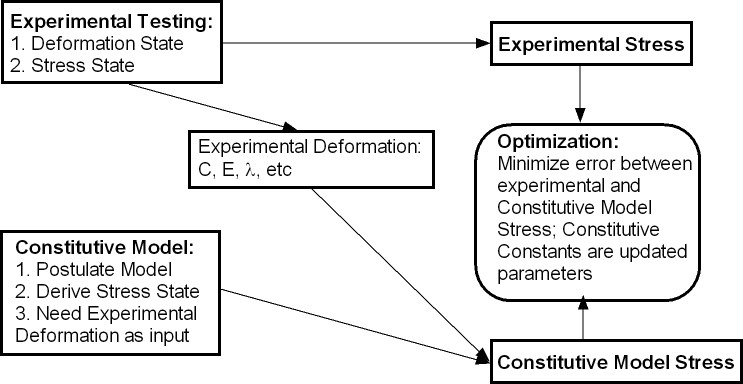
III. Deriving Experimental and Model Input for Optimization

    Many soft tissues that can be modeled as nonlinear elastic materials can often be tested as flat specimens biaxially. These includes obvious tissues such as skin, but also includes many cardiovascular tissues like blood vessels and myocardium. In this case, the tissues are subject to various stretches in one direction while holding the other direction fixed. To fit the constants, we need to perform two specific tasks that fit into the optimization model. First, we must define an experimental loading protocol that for which we can easily characterize the stress and deformation state. Since we cannot measure stress directly, but only load, we need to specify a simple loading state that we can easily characterize. In addition, we need to be able to measure the specimen deformation under the loading state as this will be used with the constitutive model to compute the stress. Second, we need to define the constitutive model we wish to fit, input the deformation state from the mechanical test, and then compute the stress for the current constants. The optimization routine will use all of these parameters to determine the constants. This procedure was illustrated in figure 1 in Section 2.

   To demonstrate fitting of a nonlinear elastic constitutive model for soft tissue, we follow a study published by Humphrey and colleages on determining passive mechanical behavior of excised myocardium:

J.D. Humphrey, R.K. Strumpf, F.C.P. Yin "Determination of a constitutive relation for passive myocardium: I. A New Functional Form", J. Biomechanical Engineering, 112:333-339, 1990.

J.D. Humphrey, R.K. Strumpf, F.C.P. Yin "Determination of a constitutive relation for passive myocardium: II. Parameter Estimation ", J. Biomechanical Engineering, 112:340-346, 1990.

To begin with, let us describe the deformation and stress state for the typical biaxial test of soft tissue shown below:

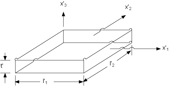
We assume that a homogeneous general biaxial state of deformation exists. Note that the specimen can deform in the third direction, that is, get thicker of thinner, in addition to deforming in plane. If we denote l1, l2 and l3 as the normal stretch in the 1, 2 and 3 direction (3 being the thickness direction), and k1 and k2 as the shearing deformation in the 1 and 2 direction (we assume no shearing occurs in the 3 direction since the specimen is very thin). The relationship between the deformed coordinate system x' and the undeformed coordinate system x can be written directly for this test as:

From the above deformation state we can directly write the deformation gradient tensor Fij as:

The Jacobian for the above deformation gradient tensor using the permutation tensor is:

Humphrey et al. make the further argument that if the specimen is thin, and the collagen fibers in the specimen are aligned with the principal testing directions, then the in plane shear stresses, k1 and k2, should be zero. This leaves the deformation gradient tensor and its determinant the Jacobian as:

In addition to F and J, we will need the right Cauchy deformation tensor C. This is calculated below:

or in matrix form:

Next, consider the stress state applied to the 2D specimen. All loads are applied normal to the specimen edge. Let the loads be denoted as p11 for the normal load in the 1 direction and p22 for the normal load in the 2 direction. The nominal stress is simply the load divided by the undeformed area. For the p11 load, the length of the specimen will be l'2, and the thickness t'. Thus, we have:

If we wish to compute the Cauchy stresses, then we use the relationship derived earlier:

which when written out in gory detail becomes:

Recalling that only the 11 and 22 terms of the nominal stress T are non-zero, and only the diagonal components of F are non-zero, we obtain the results that only the 11 and 22 terms of the Cauchy stress are non-zero and are:

We know that J is the product of the diagonal terms of F for this experimental set up. However, we also know that the material in this case is assumed to be incompressible, which means that J = 1. Applying this we obtain:

If we write the above in terms of the applied load, we have the Cauchy stress in the 1 and 2 direction as:

Thus, in summary the experimental stress and deformation states in terms of the Cauchy stress tensor and right Cauchy deformation tensor are:

 

Once we have the experimental characterization, we need to compute the stress based on the chosen constitutive model. Humphrey et al proposed the following strain energy function to characterize the pseudoelastic nonlinear behavior of passive myocardium:

where W denotes a strain energy function, I1 and I4 are invariants of the right Cauchy deformation tensor, and c1-c5 are the experimental coefficients that must be fit. Note again that this proposed constitutive law contains necessary components, namely a measure of deformation (the invariants) and the coefficients to be determined from experiment.

The invariants, which you recall are scalar functions of tensors that don't change under rotation, are defined as:

where Ni are the components of the unit vector aligned along the local muscle fiber direction. Recall that this then describes a transversely isotropic nonlinear elastic material, with the transverse isotropy due to aligned tissue fibers. For the muscle fiber direction, Humphrey et al assumed that the fibers were located in the x direction, thus the vector N would be N = (1,0,0). This would give us the final form of the invariants as:

We next need to be able to calculate the Cauchy stress for the nonlinear elastic incompressible material. Recall that the calculation of the second Piola-Kirchoff stress for a nonlinear elastic incompressible material based on a strain energy function is:

where p is the hydrostatic pressure. If we write Humphrey's form of the strain energy function in terms of C we have:

Since only the diagonal terms of C are non-zero, we will predict only that the 11, 22 and 33 componens of the 2nd PK stress will be non-zero. We can directly write these as:

We can then substitute for the right Cauchy deformation tensor components with the principal stretch components to obtain:

Next, we need to convert the 2nd PK stress components above into Cauchy stress components. The relationship of Cauchy to 2nd PK stress components is written as:

Noting that only three 2nd PK stress components are non-zero, we can have at most three Cauchy stress components that are non-zero. Thus, we have:

If we expand the Cauchy stress components in terms of the constitutive relationship we obtain:

or, upon further expansion:

At this point, it is important to remember that the 33 component of the Cauchy stress is zero. Thus, we can solve for the hydrostatic pressure as:

Substituting for p in the 11 and 22 components of the Cauchy stress gives:

 

Thus, in summary, we now have derived the quantities we need to proceed with the numerical optimization. We have the derived Cauchy stress and strain from the experimental test, and we have the Cauchy stress derived from the constitutive model. These are given below:

IV. Performing Numerical Optimization to Fit Experimental Constants

    Once we have derived the experimental stress, experimental deformation state, and constitutive model stress, we can proceed to perform the numerical optimization. Before we begin the optimization process however, it is good to have practice actually plotting data from the constitutive model for prescribed deformation states. We will do all numerical work in MATLAB. First, let us begin with code to plot the nonlinear response of passive myocardium based on the model proposed by Humphrey. We will use the following MATLAB code to do the plotting. Note that the text following the >> signs indicate MATLAB commads, while other text is a MATLAB response

>> lam1 = 1.+(0:40)/100;
>> lam2 = lam1

lam2 =

Columns 1 through 7

1.0000 1.0100 1.0200 1.0300 1.0400 1.0500 1.0600

Columns 8 through 14

1.0700 1.0800 1.0900 1.1000 1.1100 1.1200 1.1300

Columns 15 through 21

1.1400 1.1500 1.1600 1.1700 1.1800 1.1900 1.2000

Columns 22 through 28

1.2100 1.2200 1.2300 1.2400 1.2500 1.2600 1.2700

Columns 29 through 35

1.2800 1.2900 1.3000 1.3100 1.3200 1.3300 1.3400

Columns 36 through 41

1.3500 1.3600 1.3700 1.3800 1.3900 1.4000

>> for i = 1:41
sig11(i)=2.*(lam1(i)-(1./(lam1(i)^2*lam2(i)^2)))*...
(3.59-33.27*(lam1(i)-1)+2.*30.21*...
(lam1(i)+lam2(i)+(1./(lam1(i)^2*lam2(i)^2))-3))+...
lam1(i)*(2.*15.98*(lam1(i)-1)+3.*55.85*(lam1(i)-1)^2-...
33.27*(lam1(i)+lam2(i)+(1./(lam1(i)^2*lam2(i)^2))-3));
end

; Comment: sig is an array holding the Cauchy stress values for each value of the stretch ratio
; one and two arrays.

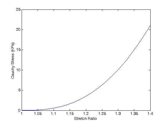
>> plot(lam1,sig11)

; Plots sig11 component versus stretch l1. When we do this we obtain:

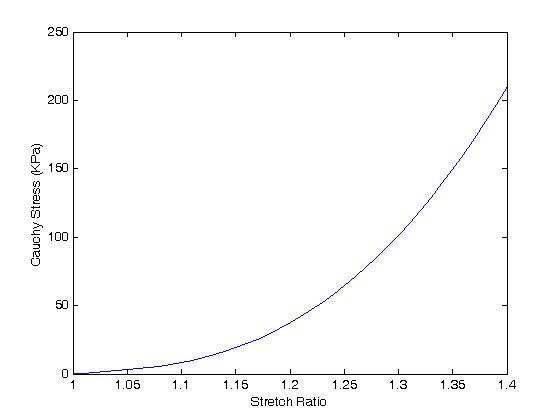
One can see the extreme nonlinearity of the passive myocardium.

As another example, consider the experimental data from Sacks and Chuong (1993) tested regions of heart muscle from the right vetnricle. They used the same strain energy function as that derived by Humphrey. They obtained the following constants:

Region                                   c1                 c2                     c3                     c4                      c5

Sinus                                    .429              15.16               .029                   -2.401                2.188

 

If we make a plot in MATLAB using the small piece of code below:

>> for i =1:41
sig11(i)=2.*(lam1(i)^2-(1./(lam1(i)^2*lam2(i)^2)))*...
(0.029-2.401*(lam1(i)-1)+2.*2.188*...
(lam1(i)^2+lam2(i)^2+(1./(lam1(i)^2*lam2(i)^2))-3))+...
lam1(i)*(2.*.429*(lam1(i)-1)+3.*15.16*(lam1(i)-1)^2-...
2.401*(lam1(i)^2+lam2(i)^2+(1./(lam1(i)^2*lam2(i)^2))-3));
end
>> plot(lam1,sig11)

we obtain:

A comparison of the two results shows:

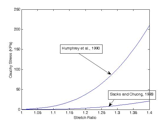
For the constants:

Region                                   c1                 c2                     c3                     c4                      c5

Sinus                                    .429              15.16               .029                   -2.401                2.188(note: these constants are reported by Humphrey, Cardiovascular Solid Mechanics, 2002)

Myocardium                         15.98            55.85              3.59                    -33.27               30.21

 

IV. Numerical Optimization to Fit Consitutive Model Constants

    To fit constants of the nonlinear elastic constitutive model for the heart, we need to perform a least squares fit between the stress from the constitutive model and that of the experimental data. As an example, let's first consider artificial data that we generate directly from the consitutive model itself, in this case the consitutive data from Sacks and Choung. Using this model, we have the following data:

Stretch ratio                         Sigma 11                      

1.04                                     .0717

1.09                                     .4400

1.14                                    1.3794

1.19                                  3.0752

1.24                                  5.6604

1.29                                  9.2419

1.34                                 13.9150

1.39                                 19.7711

We next write the optimization statement to minimize the error for these eight data points in the least squares sense as:

In MATLAB, we can use the optimization function lsqnonlin, which is a general nonlinear least squares fitting algorithm to fit the data. To do this, we first need to write a MATLAB function as shown below:

function f = heartconsfit(c)

sigex = [.0717 .4400 1.3794 3.0752 5.6604 9.2419 13.9150 19.7711];

lam1 = [1.04 1.09 1.14 1.19 1.24 1.29 1.34 1.39];

lam2 = lam1;

for i = 1:8

f(i) = 2.*(lam1(i)^2-(1./(lam1(i)^2*lam2(i)^2)))*...
(c(3)+c(4)*(lam1(i)-1)+2.*c(5)*...
(lam1(i)^2+lam2(i)^2+(1./(lam1(i)^2*lam2(i)^2))-3))+...
lam1(i)*(2.*c(1)*(lam1(i)-1)+3.*c(2)*(lam1(i)-1)^2+...
c(4)*(lam1(i)^2+lam2(i)^2+(1./(lam1(i)^2*lam2(i)^2))-3))-sigex(i);

end

Note that f(i) is actually the difference between the experimental stress (sigex(i)) and the stress computed from the constitutive model (the rest).

Once we have the function, called heartconsfit written, we have to specify an initial guess, c0, and the initial value of c. This is done in MATLAB as:

>> c = [1. 1. 1. 1. 1.]

c =

1 1 1 1 1

>> c0=[1. 1. 1. 1. 1.]

c0 =

1 1 1 1 1

Once this is set, we can then run the MATLAB least squares optimization function as follows:

>> [c,resnorm,residual]=lsqnonlin('heartconstfit',c0)
Optimization terminated: relative function value
changing by less than OPTIONS.TolFun.

c =

-0.8508 1.6236 0.3200 -1.2198 2.9316

resnorm =

6.4883e-004

residual =

0.0137 0.0012 -0.0100 -0.0096 -0.0003 0.0095 0.0099 -0.0090

Note that on the left we are the results MATLAB will return and on the right are the input of the MATLAB function and initial guess.

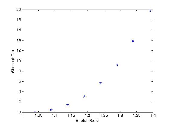
The constants we obtain (the "c" values) look much different from those with which we derived the original data. To assess the result, we first plot all the original data points in MATLAB as symbols:

segex=[.0717,.44,1.3794,3.0752,5.66,9.24,13.915,19.77];
>> stretch=[1.04,1.09,1.14,1.19,1.24,1.29,1.34,1.39];
>> plot(stretch,sigex,'marker','pentagram')

The resulting plot looks like this:

Next, we generate values for the stretch ratios in the one and two direction and overplot the graph using the constants we obtained from the optimization result.

This is done in MATLAB as follows:

>> for i=1:41
sig11(i) = 2.*(lam1(i)^2-(1./(lam1(i)^2*lam2(i)^2)))*...
(c(3)+c(4)*(lam1(i)-1)+2.*c(5)*...
(lam1(i)^2+lam2(i)^2+(1./(lam1(i)^2*lam2(i)^2))-3))+...
lam1(i)*(2.*c(1)*(lam1(i)-1)+3.*c(2)*(lam1(i)-1)^2+...
c(4)*(lam1(i)^2+lam2(i)^2+(1./(lam1(i)^2*lam2(i)^2))-3));
end
>> hold on
>> plot(lam1,sig11)

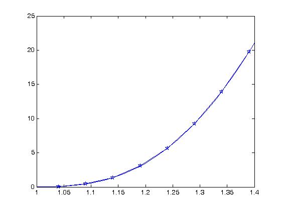
In doing this, we see an excellent fit between our optimization results and the original data points:

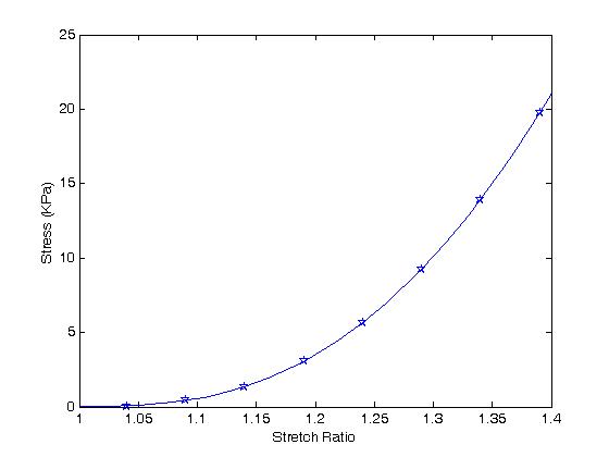
The question then becomes, how do the constants from our data fitting compare to the original constants obtained by Sacks and Chuong? We can also plot the curve for the original constants by:

>> c=[0.429 15.16 .029 -2.401 2.188]

c =

0.4290 15.1600 0.0290 -2.4010 2.1880

>> for i=1:41
sig11(i) = 2.*(lam1(i)^2-(1./(lam1(i)^2*lam2(i)^2)))*...
(c(3)+c(4)*(lam1(i)-1)+2.*c(5)*...
(lam1(i)^2+lam2(i)^2+(1./(lam1(i)^2*lam2(i)^2))-3))+...
lam1(i)*(2.*c(1)*(lam1(i)-1)+3.*c(2)*(lam1(i)-1)^2+...
c(4)*(lam1(i)^2+lam2(i)^2+(1./(lam1(i)^2*lam2(i)^2))-3));
end
>> hold on
>> plot(lam1,sig11)

When we do this, we see that the original model constants given by Sacks and Chuong (shown as the dashed red line) fit the data as well as the constants we obtained:

This result raises a very important question about nonlinear elastic constitutive model fitting, namely that the constants we can fit to these models are not unique. We have just seen this in the previous example where two very different sets of constants fit the data equally well. The questions then becomes whether we can sort out whether any set of constants obtained by an optimization process is better than another, and how do we assess whether one set of constants is superior.

The answer is not clear cut. Humphrey et al. (1990) presented their version of the Baker-Ericksen inquality for a transversely isotropic material. The Baker-Eriksen inequality, originally derived for isotropic nonlinear material constitutive equations, states that the direction of highest principal stress should correspond to the direction of highest principal stretch. Humphrey et al. (1990) stated this condition as:

In other words, for any value of the stretch ratio lamda in biaxial stretch, the constants c1-c4 should satisfy the above inequality. To see where this inquality comes from, the basic statement indicates that for a biaxial stretch, where

If the stretch is truly biaxial, then the stress in the 11 direction (if this is the stiffest direction), must be greater than or equal to the stress in the 22 direction:

If we substitute the expressions for the Cauchey stress derived from the strain energy function proposed by Humphrey and substract we get the following:

If we use the condition that the principal stretch ratios are equal, and the third stretch ratio is determined by incompressibility, we obtain:

which when separated by orders of lamda gives the result reported by Humphrey et al.

Let us plot the inequality for the range of lamda used for the fit. In MATLAB, this is done as:

>> for i = 1:41
be(i) = (3*c(2)-2*c(1)-3*c(4))+(2*c(1)-6*c(2))*lam1(i)+...
(3*c(2)+2*c(4))*lam1(i)^2+c(4)/lam1(i)^4
end

The plot for the original constants gives:

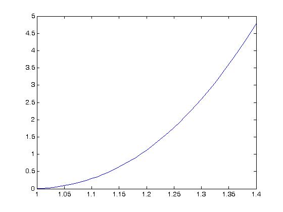
we can see that the original parameters satisfy this inequality as all values are greater than or equal to zero.

If we plot the same inequality for the constants we obtain using the MATLAB fit, we obtain:

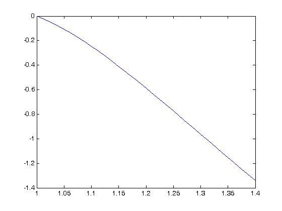
which unfortunately suggests that the results we obtained are not satisfactory.

Our next questions is whether it is possible to impose directly the stability constraint proposed by Humphrey directly in the optimization. The answer is that it is possible with MATLAB. We can do this using the optimization routine fmincon. In this case, we have to write one MATLAB function to calculate the least squares problem directly and one MATLAB function to implement the constraint. For the objective function we have the MATLAB function as follows:

For fmincon we write a MATLAB function that evaluates the objective function as follows:

function f = heartfitconstraint(cf)

sigex = [.0717 .4400 1.3794 3.0752 5.6604 9.2419 13.9150 19.7711];

lam1 = [1.04 1.09 1.14 1.19 1.24 1.29 1.34 1.39];

lam2 = lam1;

f = 0.0;

for i = 1:8

f = f + (2.*(lam1(i)^2-(1./(lam1(i)^2*lam2(i)^2)))*...
(cf(3)+cf(4)*(lam1(i)-1)+2.*cf(5)*...
(lam1(i)^2+lam2(i)^2+(1./(lam1(i)^2*lam2(i)^2))-3))+...
lam1(i)*(2.*cf(1)*(lam1(i)-1)+3.*cf(2)*(lam1(i)-1)^2+...
cf(4)*(lam1(i)^2+lam2(i)^2+(1./(lam1(i)^2*lam2(i)^2))-3))-sigex(i))^2;

end

We then need to write a second function that evaluates the constraint on the model coefficients. This follows:

function [c,ceq] = heartbehconstraint(cf)

lam1 = [1.04 1.09 1.14 1.19 1.24 1.29 1.34 1.39];

for i = 1:8

c(i) = -3*cf(2)+2*cf(1)+3*cf(4)-(2*cf(1)-6*cf(2))*lam1(i)-...
(3*cf(2)+2*cf(4))*lam1(i)^2-cf(4)/lam1(i)^4

end

ceq =[];

end

We then run the optimization routine fmincon at the MATLAB prompt as:

[cf,fval]=fmincon('heartfitconstraint',cf0,[],[],[],[],[],[],'heartbehconstraint')

where the empty brackets represent quantities that are not needed for the minimization. The results are:

cf =

1.5318 1.8791 -0.0670 -1.8126 2.9642

Now let's check the stress strain curve with these coefficients. We we plug these coefficients in to obtain:

>> for i=1:41
sig11(i)=2.*(lam1(i)^2-(1./(lam1(i)^2*lam2(i)^2)))*...
(cf(3)+cf(4)*(lam1(i)-1)+2.*cf(5)*...
(lam1(i)^2+lam2(i)^2+(1./(lam1(i)^2*lam2(i)^2))-3))+...
lam1(i)*(2.*cf(1)*(lam1(i)-1)+3.*cf(2)*(lam1(i)-1)^2+...
cf(4)*(lam1(i)^2+lam2(i)^2+(1./(lam1(i)^2*lam2(i)^2))-3));
end
>> plot(lam1,sig11)
>> hold on
>> plot(stretch,segex,'marker','pentagram')

Once again, we see that the optimization process, this time using the MATLAB general nonlinear programming function fmincon with the stability constraint, fits the "manufactured" Sacks and Chuong data very well. Next, we plot the constraint versus the stretch ratio for material stability. In MATLAB:

for i = 1:41
be(i) = (3*cf(2)-2*cf(1)-3*cf(4))+(2*cf(1)-6*cf(2))*lam1(i)+...
(3*cf(2)+2*cf(4))*lam1(i)^2+cf(4)/lam1(i)^4;
end

>> plot(lam1,be)

We obtain the plot:

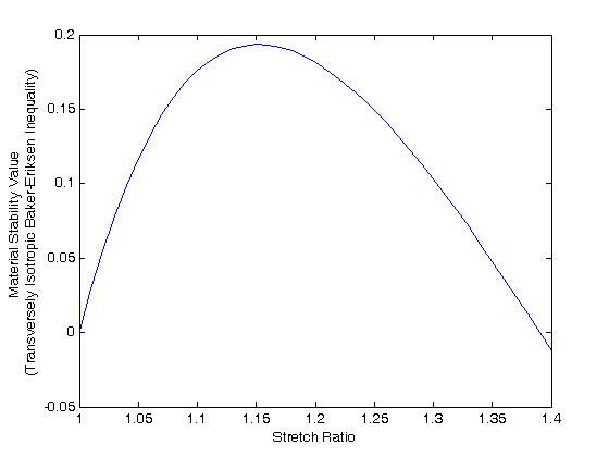
Note that the material stability constraint is satisfied up through the stretch ration 1.4. This was the highest stretch ratio used for the data fit in the optimization run. The constraint is violated for a stretch ratio of 1.41, which was not covered by the constraint.

IV. Performing Numerical Optimization to Fit Experimental Constants

    In this section we have demonstrated how nonlinear hyperelastic consitutive constants can be fit for biaxial test specimens using optimization routines in MATLAB. In this scenario, one must first choose a test specimen with a simplified geometry such that the experimental stress state and deformation state can be easily calculated analytically. Thus, the procedures are:

1. Analytically calculate stress and deformation state

2. Substitute experimental deformation state into constitutive equation to compute model stress

3. Use Numerical Optimization techniques to calculate nonlinear elastic coefficients