I. Overview

       Determining and fitting constitutive models for biological tissues is important in its own right for many applications. Among these are understanding structure-function relationships for biological tissues in normal physiologic circumstances and how these structure-function relationships may change due to disease or aging. One prime example was shown in the overview for ateries where stiffness increases due to chronic hypertension. In addition, constitutive models provide a quantitative way for us to compare the function of normal and engineered tissues. However, a major reason for establishing constitutive models is so that we can actually solve the equilibrium problem as discussed in chapter 6 on nonlinear elastic constitutive equations. Solving equilibrium problems is critical in biosolid mechanics since it will enable us to determine stress and strain distributions within tissues. Determining stress/strain distributions is necessary for understanding tissue failure under mechanical loads and for relating local stress and strain distributions of physiological processes. In general, we cannot solve the stress equilibrium problem directly without making assumptions about small versus large strain and constitutive models. Even we we establish a constitutive model, however, it is generally not possible to solve the governing equilibrium problem for most realistic 3D problems and numerical approximation methods most be used. Solving equil

      By far the most popular numerical method for solving stress equilibrium problems is the finite element method. The termed "finite element" is used to denote the fact that the original 3D geometry is broken up into a finite set of small elements. These elements represent a mathematical approximation to the displacement field that is usually a polynomial with unknown coefficients. Substituting this polynomial approximation into the original partial differential stress equilibrium equations basically converts these PDE into a set of algebraic equations that are solved using numerical methods.

     Due to the amount of work involved in writing computer code to solve solid mechanics problems using finite elements, a number of commercially available codes have been developed. Among the most widely known of these are NASTRAN, ABAQUS, MARC, ANSYS and FEMLAB. Basically, all of these codes require the user to enter the original 3D geometry of the stress equilbrium problem, along with boundary conditions and constitutive models. The commercial code then generates the numerical approximation to the stress equilibrium PDE and solves the corresponding system of linear algebra equations. Even if the initial problem is nonlinear due to large deformation and/or nonlinear material properties, the numerical approximation breaks it down into a set of linear equations due to additional approximations.

    As mentioned, it is infrequent that one desiring to solve a stress equilibrium problem will write their own code, but instead will used commercially available codes. However, even when using commercial codes it is important to have an understanding of what finite elements are and what approximations are made to better understand the use of commercial codes. Therefore, we will provide a brief overview to finite element approximations for a simple linear elastic 1D case, and then illustrate how to run a nonlinear analysis using isotropic strain energy functions in the commercial code ABAQUS.

II. 1D Linear Finite Element Methods

   To illustrate the basic tenets of finite element methods, we will start with a 1D linear elastic stress analysis problem. We begin with the 1D differential equation for stress equilibrium:

To create the finite element approximation, we must first multiply the above one dimensional equilibrium problem by a "virtual" displacement v, and then integrate over the length of the 1D continuum which we denote as L:

Since the area of the bar is assumed to be a constant "A", this accounts for the 3 dimensions of the problem. Note that the function v is also called a "test" function and the integral of the stress equilibrium problem is also called the "weak" form of the solution with the original differential equation being called the "strong" form. At this point, we can apply the 1D linear elastic constitutive equation:

With the small strain displacement relation:

If we substitute both the linear elastic constitutive equation and the strain displacement relation into the weak form integral we obtain:

Next, we apply integration by parts to the above equation to obtain:

where the right hand term represents a boundary condition on the virtual displacement and the stress at the boundary 0 and L. The virtual displacement is such that when the real displacement u has a fixed value, then v has the value of 0. Thus, if we assume that the left hand of the bar is fixed as shown below:

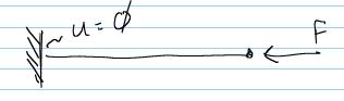
Then we have:

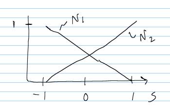
At this point, we now make the approximation of both the "real" displacement field u and the "virtual" displacement field v using a polynomial. We will use an isoparametric polynomial. The polynomial, often called a shape function, is created such that the displacement on one side of the element is u1 and the displacement on the other side of the element is u2. The shape functions are given below:

The shape functions are given in computational coordinates s, which for the isoparametric element must range from -1 to 1. A graph of the shape functions is shown below:

Then, the displacement field within the element (u for the real displacement, v for the virtual displacement) may be represented as:

In addition to approximating the real and virtual displacements using the isoparametric shape functions, we also approximate the phyiscal coordinates x using the same shape functions. This is actually where the definition "isoparametric" stems from. This, the coordinates are given as:

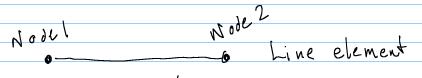
Were the 1D element has two nodes (points at the end of the element) at which u1, v1,x1 and u2, v2,x2 are defined. This element is shown below:

At this point, we need to relate the computational coordinates s to the physical coordinates x, as well as derivatives with respect to s to derivatives with respect to x. This can be done through the chain rule as:

Note that the quantity ds/dx can be directly calculated from the isoparametric approximation of the coordinates given above:

We also need to know the differential length dx for the integral in terms of ds, so that we can convert the integral over the bar length L into an integral over the isoparametric element s. Again, we can apply the chain rule:

At this point, it is useful to collect all the approximations that we have made and substitute these into the integral as:

We can rewrite all of the above in matrix vector forms to achieve:

Now we have that the integral over the whole bar length can actually be broken up into the sum of integrals over each element. At this point it is important to note that v1,v2,u1,u2,A,E,x1,x2 are all constants over the integration over s and thus the final integral may be written as:

In finite elements, the inner matrix term is called the element stiffness matrix. Now, we will make the same approximation for the boundary term. First note that the term EAdu/dx actually represents a traction force that we can simply call f. This give us the boundary term as:

If we apply the vector interpolation for v into the above we obtain:

The vector contianing f on the right hand side is often called the load vector.

Thus, our original differential equation and subsequent integral weak form has been converted into a system of linear equations as:

Since the vector quantity containing v1 and v2 multiplies both the stiffness matrix and the load vector, we may remove it from the equation to leave us with:

In the above equation, E, A, and L must be given as do f. These represent the constitutive model and the boundary conditions. If we denote the term with EA/L as the element stiffness matrix ke, the load vector on the right as the element load vector f, and the element displacement vector as u, then we can write the sum of each term as their global representation:

Then, finally, the set of linear equations we must solve becomes:

This set of linear equations is the fundamental equations that are solved in ALL finite element approximations, no matter if they are time dependent or nonlinear. That is because in these instances we end up making approximations for time or nonlinearity in steps where each step boils down to solving a system of linear equations. The theory behind these approximations are beyond the scope of this course.

Also note that the summation used to obtain the global equations is not a simple summation, but rather a complex assembly of elements to a global model based on what nodes of an element are connected to what other nodes. Thus, to define a finite element computational model, we need to enter the following:

1. Node locations and element connectivity (defines the geometry of the model)

2. Constitutive Model

3. Boundary Conditions

4. Strain Displacement Relationship (large or small strain)

Once these factors are entered, the commercial code can solve the finite element approximation of the original stress equilibrium problem. In the next section, we give an example for nonlinear modeling using ABAQUS.

III. Example 3D Simple Nonlinear Elastic Finite Element Model in ABAQUS

   To illustrate how we use commercial codes to solve realistic biosolid problems in practice, we will use a simple 3D model with nonlinear elastic problems. Consider the following geometry that was created in the finite element pre-processing software Hypermesh:

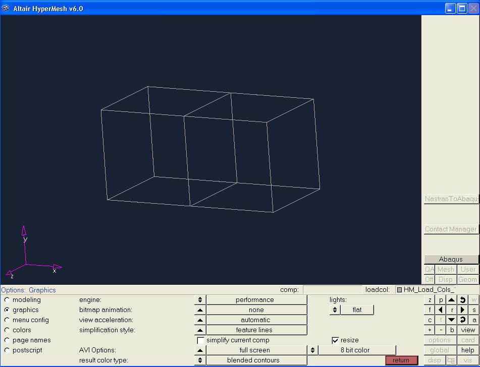
This is simply a two element model in 3D. The resulting input file for ABAQUS created using this geometry is shown below:

** Human Vena Cava Data
** ABAQUS Input Deck generated by HyperMesh version2.00a
** Template: ABAQUS/STANDARD
**
*HEADING
ABAQUS input file from HyperMesh
*SYSTEM
*NODE
10.000000000.000000000.00000000
21.000000000.000000000.00000000
32.000000000.000000000.00000000
40.000000001.000000000.00000000
51.000000001.000000000.00000000
62.000000001.000000000.00000000
70.000000000.000000001.00000000
81.000000000.000000001.00000000
92.000000000.000000001.00000000
100.000000001.000000001.00000000
111.000000001.000000001.00000000
122.000000001.000000001.00000000
*ELEMENT, TYPE=C3D8RH, ELSET=auto1
1 1 4 10 7 2 5 11 8
2 2 5 11 8 3 6 12 9
*SOLID SECTION, ELSET=auto1, MATERIAL=auto1
**HMCOLOR, COMP=auto1, COLOR=1
*MATERIAL, NAME=auto1
*HYPERELASTIC, TEST DATA INPUT, POLY, N=1
*UNIAXIAL TEST DATA
0.,0.
1.,.05
2.,.1
5.,.15
10.,.2
20.,.225
40.,.25
*STEP,NLGEOM,INC=50
HUMAN VENA CAVA
*STATIC
*CLOAD, OP=NEW
3 11.00000000
6 11.00000000
9 11.00000000
12 11.00000000
*BOUNDARY, OP=NEW
1 1 0.00000000
1 2 0.00000000
1 3 0.00000000
4 1 0.00000000
4 2 0.00000000
4 3 0.00000000
7 1 0.00000000
7 2 0.00000000
7 3 0.00000000
10 1 0.00000000
10 2 0.00000000
10 3 0.00000000
*EL PRINT, POSITION=CENTROIDAL, FREQUENCY=1, SUMMARY=YES
*NODE PRINT, FREQUENCY=1, SUMMARY=YES, TOTALS=YES
*EL FILE, POSITION=CENTROIDAL, FREQUENCY=1
S, DG, E, SINV
*NODE FILE, FREQUENCY=1
U
*END STEP

Let's breakdown the portions of the input file. First, the geometry of the model is defined in terms of the nodal coordinates and the element connectivity in the sections given below:

 

GEOMETRY

*NODE
10.000000000.000000000.00000000
21.000000000.000000000.00000000
32.000000000.000000000.00000000
40.000000001.000000000.00000000
51.000000001.000000000.00000000
62.000000001.000000000.00000000
70.000000000.000000001.00000000
81.000000000.000000001.00000000
92.000000000.000000001.00000000
100.000000001.000000001.00000000
111.000000001.000000001.00000000
122.000000001.000000001.00000000
*ELEMENT, TYPE=C3D8RH, ELSET=auto1
1 1 4 10 7 2 5 11 8
2 2 5 11 8 3 6 12 9
*SOLID SECTION, ELSET=auto1, MATERIAL=auto1

Here *NODE is the ABAQUS definition of node coordinates that are given as x,y and z. *ELEMENT, ... tells ABAQUS the type of element we are using, which in our finite element derivation is really the type of polynomial approximation we are using to describe the displacement field. In this case, we are using a reduced integration 8 node element. This is a special type of polynomial approximation used to deal with incompressible nonlinear elastic materials. Also, in 3D these are 8 node elements, so there are 8 numbers that represent how the elements are connected. Finally, *SOLID SECTION tells ABAQUS that this is a 3D material and points to the constitutive data with MATERIAL = auto1.

CONSTITUTIVE DATA

*HYPERELASTIC, TEST DATA INPUT, POLY, N=1
*UNIAXIAL TEST DATA
0.,0.
1.,.05
2.,.1
5.,.15
10.,.2
20.,.225
40.,.25

Here *HYPERELASTIC tells ABAQUS we are dealing with a nonlinear elastic material. TEST DATA INPUT tells ABAQUS means that we are using test data input to fit the polynomial strain energy function. This is really similar to a Neo Hookean model. We can input the model constants directly into ABAQUS as well.

STRAIN DISPLACEMENT DATA

*STEP,NLGEOM,INC=50

This is where we tell ABAQUS that we are dealing with large strains, and thus using the large strain tensor versus the small strain tensor. ABAQUS uses NLGEOM to denote the use of the large strain tensor.

BOUNDARY CONDITIONS

*STATIC
*CLOAD, OP=NEW
3 11.00000000
6 11.00000000
9 11.00000000
12 11.00000000
*BOUNDARY, OP=NEW
1 1 0.00000000
1 2 0.00000000
1 3 0.00000000
4 1 0.00000000
4 2 0.00000000
4 3 0.00000000
7 1 0.00000000
7 2 0.00000000
7 3 0.00000000
10 1 0.00000000
10 2 0.00000000
10 3 0.00000000

The last data needed by ABAQUS to solve the problem is the boundary condition data. Here we can specify both force and displacement boundary conditions. *STATIC tells ABAQUS that there are no time dependent forces. *CLOAD is the definition for an applied force. *BOUNDARY denotes conditions on displacement used by ABAQUS. Note that in reality for numerical problems we typically cannot get a solution without specification of some displacement boundary conditions.

OUTPUT

*EL PRINT, POSITION=CENTROIDAL, FREQUENCY=1, SUMMARY=YES
*NODE PRINT, FREQUENCY=1, SUMMARY=YES, TOTALS=YES
*EL FILE, POSITION=CENTROIDAL, FREQUENCY=1
S, DG, E, SINV
*NODE FILE, FREQUENCY=1
U

 

Note that ABAQUS will be happy to go through and solve our defined equilibrium problem without giving us much output. We typically want to know the displacements which are calculated at the nodes and the stress and strain data which is calculated somewhere within the element. *EL PRINT prints those quantitites associated with the elements. *NODE PRINT prints those quantitites associated with the nodes, typically displacements in the static case and velocities and accelerations in the dynamic case

IV. Summary

   In summary, we have provided a very brief introduction to the use of finite element methods to solve the governing stress equilibrium problems. Finite element methods are numerical techniques that can be used to model a biosolid mechanics problem. This finite element input data draws on all the components we talked about in class, including boundary conditions, constitutive models and stress equilibrium problems.