I. Overview

    As noted in the last section, the quasilinear viscoelastic (QLV) constitutive model is perhaps the most common viscoelastic constitutive models used to characterize biological soft tissues. It has the capability of modeling materials with time dependent viscoelastic behavior that undergo large deformation. As with any constitutive equation, we must be able to fit the constants in the model. To fully fit this constitutive model, we need to perform time dependent stress relaxation tests and fit the constants of the function that characterizes stress relaxation as well as large deformation.

   Difficulties in fitting the quasilinear model for stress relaxation tests were previously complicated by the need to have a very fast ramp to the applied strain. Recently, Abramowitch and Woo (2004) published a method to fit the QLV model using a ramp time with finite speed. This reference is:

Abramowitch, SD and Woo, SLY (2004) "An improved method to analyze the stress relaxation of ligaments following a finite ramp time based on the quasi-linear viscoelastic theory", Journal of Biomechanical Engineering, 126:92-97

However, utilizing the reduced relaxation function proposed by Fung can be quite complicated. Therefore, we adopt a simpler reduced relaxation function proposed by Toms et al. (2002):

Toms, SR, Dakin, GJ, Lemons, JE, and Eberhardt, AW (2002) "Quasi-linear viscoelastic behavior of the human periodontal ligament", J. Biomechanics, 35:1411-1415.

In this section, we will repeat the work of Abramowitch and Woo and show how their method may be used with MATLAB optimization routines to fit QLV theory. At the end of the section, you should:

1. Be better able to understand QLV theory
2. Understand the experimental tests necessary to determine QLV constants
3. Be able to fit QLV constants using MATLAB optimization routines

II. QLV Theory Revisited

    As noted previously, QLV theory models the viscoelastic response of a material based on a stress relaxation function and the instantaneous stress resulting from a ramp strain as:

where s(t) is the stress at any time t, se(e) is the stress corresponding to an instanteous strain, G(t) is the reduced relaxation function representing the stress of the material divided by the stress after the initial ramp strain Note that * represents the convultion of G and se(e), which is G(t) multiplied by se(e) and then integrated over time. G(t) is defined as:

The complete stress history at any time t is then the convolution integral:

where G is the reduced relaxation function,   represents the instantaneous elastic response, and   is the strain history. We can assume that t starts at 0 instead of negative infinity for the experimental situaiton. The reduced relaxation function proposed by Toms et al is:

where a,b,c,d,g,h are all constants to be determined experimentally.

The instantaneous stress response is assumed to be represent through the nonlinear elastic relationship:

Is the nonlinear elastic function, A and B are constants that must be determined by experiment.

where A and B are constants to be fit with experimental data. Thus, in this QLV one dimensional model there are eight constants to be determined: a,b,c,d,g,h,A,B.

II. QLV Theory Implemented for a Ramp strain

    The ramp strain for determining stress relaxation is defined as:

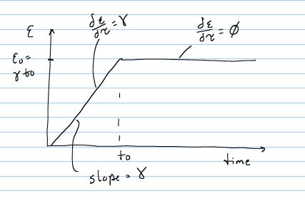
From t = 0 to t = t0, there is constant linear increase in strain with slope g, and the total strain at any time during the ramp is simply gt. Thus, for this time frame the strain time history is:

Over the time period t = t0 to the end of the testing period, the strain level is held constant and thus:

The other parameters we need for the response to the ramp strain are the derivative of the nonlinear elastic function with respect to strain. This is readily calculated as:

We can thus substitute for the strain history and the instantaneous stress reponse into the QLV model to obtain the stress history from 0 to before t0 and from t0 to the end of the test period. From 0 to before t0 we have:

were note that we have substituted e = gt for the strain in the nonlinear elastic response and have pulled the constants A,B, t1, and t2 that are not under time dependent have been pulled out of the integral. Note the stress response from t0 to the end of the experiment includes the stress history up to t0 plus the stress history from t0 onward. However, since the strain rate from t0 onward is zero, we are simply left with:

Thus we have a representation for the stress history up to time t0 and from t0 afterward.

We can analytically integrate the above integrals to obtain:

for 0 < t < t0 and for t > t0 we obtain:

If we apply the integration limits we obtain:

for t < t0 and for t > t0 we have:

Once this analytical form is known, we can then plot results and perform optimization in MATLAB.

III. Evaluating and Plotting Results from Periodontal Ligament QLV data

    As with the nonlinear elastic curve fitting, our first step into fitting constants for the QLV model is to actually evaluate the QLV function for specified data. This is important because we must correctly evaluate stress calculated from QLV theory as one part of evaluating our objective function in the fit. Let us consider constants reported by Toms et al for the periodontal ligament. One such set of constants is:

A = .014 MPa

B = 8.41

gam = 0.15%/second or .0015/second

a = .0897

b = .1548

c = .1093

d = .0038

g = .7852

h = .0000352

t0 = 18.4 seconds

(Note that gam and t0 are adopted from Abramowitch and Woo).

We can use these constants in the analytical form dervied above to plot the stress relaxation response in MATLAB.

We first enter the constants in MATLAB:

>> A = .014;
>> B = 8.41;
>> a = .0897;
>> b=.1538;
>> c=.1093;
>> d=.0038;
>> g=.7852;
>> h=.0000352;
>> t0=18.4
>> gam=.0015;
>> t1=(0:184)/10.;
>> t2=(19:3619);

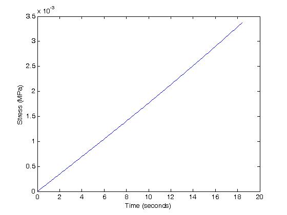
where t1 is the full time array going from 0 to the ramp up time of 18.4 seconds in increments of 0.1 seconds, and t2 if the array going from the ramp up time to 3600 seconds in increments of 1 second. We next enter the analytical expression for the stress into MATLAB in a for loop, noting the exp(x) is the exponential function in MATLAB. For t < t0 we have:

for i = 1:185
sig1(i) = A*B*gam*(a*exp(B*gam*t1(i))/(b+B*gam)+c*exp(B*gam*t1(i))/(d+B*gam)+g*exp(B*gam*t1(i))/(h+B*gam))-...
A*B*gam*(a*exp(-b*t1(i))/(b+B*gam)+c*exp(-d*t1(i))/(d+B*gam)+g*exp(-h*t1(i))/(h+B*gam));
end
>> plot(t1,sig1)

Which gives us the stress during the ramp up strain versus time plot:

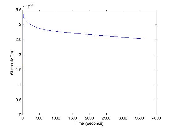
For t > t0, we have:

>> for i = 1:3601
sig2(i)=A*B*gam*(a*exp(-b*t2(i))*exp(b*t0+B*gam*t0)/(b+B*gam)+c*exp(-d*t2(i))*exp(d*t0+B*gam*t0)/(d+B*gam)...
+g*exp(-h*t2(i))*exp(h*t0+B*gam*t0)/(h+B*gam))...
-(A*B*gam*(a*exp(-b*t2(i))/(b+B*gam)+c*exp(-d*t2(i))/(d+B*gam)+g*exp(-h*t2(i))/(h+B*gam)));
end
>> plot(t2,sig2)
>> hold on
>> plot(t1,sig1)

Which gives us the following stress versus time plot:

IV. Fitting the Periodontal QLV data

    Abramowitch and Woo (2004) proposed a method for fitting QLV constants in which the stress from the ramp up strain and the stress following the ramp up strain are consider as additive parts to the objective function. If we let be the experimental strain up to ramp up and be the experimental stress after ramp up, we have the following objective function:

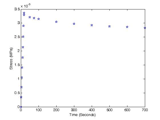
where the first term represents the ramp up stress and the second term represents the stress from ramp up until a long period reaching equilbrium. To illustrate the fitting procedure, we will again generate data from the model at specific time points. We will use the following as input:

tramp = [0 2. 4. 6. 8. 10. 12. 14. 16. 18.];
sigramp = [0 .0003 .0007 .0010 .0014 .0018 .0021 .0025 .0029 .0033];

tinf = [19.,50.,75.,100.,200.,300.,400.,500.,600.,700.];
siginf =[.0034 .0032 .0032 .0031 .0030 .0030 .0029 .0029 .0028];

where tramp represents the first part of the objective function for the ramp strain and tinf represents the second part of the stress during the relaxation. Plotting the experimental data gives:

 

For the optimization using fmincon, we make the following associations:

c(1) = A
c(2) = B
c(3)=a
c(4)=b
c(5)=c
c(6)=d
c(7)=g
c(8)=h

We use fminunc in MATLAB for the optimization fit, which is similar to fmincon but without constraints. In fact, fminunc works on unconstrained nonlinear minimization problems. We again need to write a MATLAB function that will evaluate the objective function, which I have called qlvfitun.m. This is given below:

function f = qlvfitun(c)

t0 = 18.4;
gam = .0015;

tramp = [0. 2. 4. 6. 8. 10. 12. 14. 16. 18.];
sigramp = [0. .0003 .0007 .0010 .0014 .0018 .0021 .0025 .0029 .0033];

tinf = [19. 50. 75. 100. 200. 300. 400. 500.];
siginf =[.0034 .0032 .0032 .0031 .0030 .0030 .0029 .0029];

f1 = 0.
f2 = 0.

for i = 1:10

t1(i)=tramp(i);

f1 = f1+(c(1)*c(2)*gam*(c(3)*exp(c(2)*gam*t1(i))/(c(4)+c(2)*gam)+c(5)*exp(c(2)*gam*t1(i))/(c(5)+c(2)*gam)+c(7)*exp(c(2)*gam*t1(i))/(c(8)+c(2)*gam))-...
c(1)*c(2)*gam*(c(3)*exp(-c(2)*t1(i))/(c(4)+c(2)*gam)+c(5)*exp(-c(6)*t1(i))/(c(6)+c(2)*gam)+c(7)*exp(-c(8)*t1(i))/(c(8)+c(2)*gam))-sigramp(i))^2;

end

icount = 0;

for i = 1:8

;icount = icount+1;
t2=tinf(i);
sig2=siginf(i);

f2 = f2+(c(1)*c(2)*gam*(c(3)*exp(-c(4)*t2)*exp(c(4)*t0+c(2)*gam*t0)/(c(4)+c(2)*gam)+c(5)*exp(-c(6)*t2)*exp(c(6)*t0+c(2)*gam*t0)/(c(6)+c(2)*gam)...
+c(7)*exp(-c(8)*t2)*exp(c(8)*t0+c(2)*gam*t0)/(c(8)+c(2)*gam))...
-(c(1)*c(2)*gam*(c(3)*exp(-c(4)*t2)/(c(4)+c(2)*gam)+c(5)*exp(-c(6)*t2)/(c(6)+c(2)*gam)+c(7)*exp(-c(8)*t2)/(c(8)+c(2)*gam)))-sig2)^2;

end

f = f1+f2

end

 

Then, to run the optimization routine we do as before:

[c,fval,exitflag]=fminunc('qlvfitun',c0)

where c are the values of the coefficients, fval is the value of the objective function, and exitflag gives us the reason the algorithm exited. c0 is again an initial guess.

The results are:

c =

0.5344 0.4967 -0.0249 0.0399 0.1226 0.1266 0.4358 0.0002

fval =

2.4127e-008

exitflag =

1

Exitflag 1 indicates that the algorithm converged to a solution, with the following coefficients:

A = .534 MPa
B = 0.4967
a = -.0249
b = .0399
c = .1226
d = .1266
g = .4358
h = .0002

If we plug these values into the stress result and plot the answer using the following MATLAB code:

>> tinf = [19. 50. 75. 100. 200. 300. 400. 500.];
siginf =[.0034 .0032 .0032 .0031 .0030 .0030 .0029 .0029];
>> tramp = [0. 2. 4. 6. 8. 10. 12. 14. 16. 18.];
sigramp = [0. .0003 .0007 .0010 .0014 .0018 .0021 .0025 .0029 .0033];
>> plot(tinf,siginf,'marker','pentagram')
>> hold on
>> plot(tramp,sigramp,'marker','pentagram')
>> c=[0.5344 0.4967 -0.0249 0.0399 0.1226 0.1266 0.4358 0.0002
]

c =

0.5344 0.4967 -0.0249 0.0399 0.1226 0.1266 0.4358 0.0002

>> t1=(0:185)/10.;
>> t2=(19:3619);
>> t0=18.4;
>> gam=.0015;


>> for i = 1:186
sig(i)=c(1)*c(2)*gam*(c(3)*exp(c(2)*gam*t1(i))/(c(4)+c(2)*gam)+c(5)*exp(c(2)*gam*t1(i))/(c(5)+c(2)*gam)+c(7)*exp(c(2)*gam*t1(i))/(c(8)+c(2)*gam))-...
c(1)*c(2)*gam*(c(3)*exp(-c(2)*t1(i))/(c(4)+c(2)*gam)+c(5)*exp(-c(6)*t1(i))/(c(6)+c(2)*gam)+c(7)*exp(-c(8)*t1(i))/(c(8)+c(2)*gam));
end
>> hold on
>> plot(t1,sig)
>> hold on

>> for i = 1:3601
sig2(i)=c(1)*c(2)*gam*(c(3)*exp(-c(4)*t2(i))*exp(c(4)*t0+c(2)*gam*t0)/(c(4)+c(2)*gam)+c(5)*exp(-c(6)*t2(i))*exp(c(6)*t0+c(2)*gam*t0)/(c(6)+c(2)*gam)...
+c(7)*exp(-c(8)*t2(i))*exp(c(8)*t0+c(2)*gam*t0)/(c(8)+c(2)*gam))...
-(c(1)*c(2)*gam*(c(3)*exp(-c(4)*t2(i))/(c(4)+c(2)*gam)+c(5)*exp(-c(6)*t2(i))/(c(6)+c(2)*gam)+c(7)*exp(-c(8)*t2(i))/(c(8)+c(2)*gam)));
end
>> plot(t2,sig2)

we obtain:

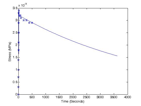
which shows a reasonable fit to the experimental data. If we had used more data points, we could possibly obtain a better fit.

V. QLV Theory: Connection of Nonlinear Elasticity with Stress Relaxation and Creep

    The QLV theory presented here uses a 1D constitutive model to describe the instantaneous nonlinear elastic response of the material. However, within the framework of QLV theory, it is possible to utilize nonlinear elastic strain energy functions with creep or stress relaxation functions to capture the instantaneous nonlinear anisotropic deformation. This expanded application of QLV theory has been discussed in a number of papers, see for example Tonuk and Silver-Thorn (2004), Li et al. (2006) and Bischoff (2006). In this case, one essentially proposes a time dependent strain energy function that is a typical nonlinear elastic strain energy function multiplied by a time dependent stress relaxation function (since we are calculating stress from strain). This is given below as:

                                                                       

where is the typical strain energy function used for nonlinear elasticity. Let us next consider how to use this in the context of QLV theory. The components we need to calculate stress using QLV are the reduced relaxation function G(t), and the derivative of the stress with respect to the strain. To calculate the latter using an incompressible strain energy function we proceed as follows:

                                      

If we substitute the above result into a QLV form for the stress, we have:

                         

This is the general form of stress for QLV theory when we assume the existence of a general strain energy function for the instantaneous elastic response. Now let us propose a specific form of strain energy function, reduced relaxation function and strain history for a viscoelastic tissue specimen. Let us first propose to use an incompressible three-parameter Mooney-Rivlin strain energy function proposed by Li et al. (2006) for soft tissues in the pubic symphysis:

                                                 

which expanded in 3D gives:

 

To simplify, we will assume we are calculating the S11 component of the second PK stress tensor. We also assume that there are no shear strains during the deformation, and that the material is incompressible. We assume furthermore that we will apply a uniaxial stretch in the 1 direction denoted as l1. Using incompressiblility, and the stretch ratio, we can calculate the complete right Cauchy deformation gradient tensor as:

                                  

Which gives us the right Cauchy Deformation tensor as:

                                  

We can then simplify the strain energy function for this deformation state as:

                     

Let us look again at the derivative at the derivative of the stress with respect to the strain time the strain rate. Considering that only the normal components of the finite strain tensor are non-zero, we have:

Thus, we first need to compute 3 second order derviatives of the strain energy function. We can do this in the symbolic manipulator in MATLAB as:

>> syms e11
>> syms c11 c22 c33 c10 c01 c11
>> syms C11 C22 C33 c10 c01 c11
>> w = c10*(C11+C22+C33-3)+c01*(C11*C22+C11*C33+C22*C33-3)+...
c11*(C11+C22+C33-3)*(C11*C22+C11*C33+C22*C33-3)

w =

c10*(C11+C22+C33-3)+c01*(C11*C22+C11*C33+C22*C33-3)+c11*(C11+C22+C33-3)*(C11*C22+C11*C33+C22*C33-3)

We first differentiate W with respect to C11:

>> wc11 = diff(w,'C11')

wc11 =

c10+c01*(C22+C33)+c11*(C11*C22+C11*C33+C22*C33-3)+c11*(C11+C22+C33-3)*(C22+C33)

Then, to take the second derviative, we sequentially differentiate with respect to C11, C22 and then C33:


>> wc11c11 = diff(wc11,'C11')

wc11c11 =

2*c11*(C22+C33)


>> wc11c22 = diff(wc11,'C22')

wc11c22 =

c01+c11*(C11+C33)+c11*(C22+C33)+c11*(C11+C22+C33-3)


>> wc11c33 = diff(wc11,'C33')

wc11c33 =

c01+c11*(C11+C22)+c11*(C22+C33)+c11*(C11+C22+C33-3)

We thus have for the 2nd PK stress as a function of time:

To calculate the derivate of the derivative of the inverse of C. For this defomration state, C is a diagonal matrix. Thus, the inverse of C is:

Thus, the derivative of the inverse of C is:

Thus, we have the 2nd PK stress as a function of time as:

For the stress relaxation function, many researchers have chosen a prony series which has the form:

where d1 and d2 represent short and long term relaxation magnitudes, and t1 and t2 represent short and long term relaxation time constants.

As in the case of any step strain test, the integral would be split into the time it takes to ramp up the strain, and then the time past this ramp time. We would use the typical ramp strain test:

where g is again the strain rate up to t0. Thus, the integral up to t0 would look like:

The integral after t0 would look like:

To fit this data, we would need to find the hydrostatic pressure p from the fact that S22 = 0. We would also need to calculate the strain rate in the 22 and 33 directions based on taking the
derivative of the incompressibility constrain with respect to time. We would then fit experimental data from d1,d2,t1,t2,c01, and c11.

VI. Modeling strain rate dependence using a combined elastic and viscous potential

    An alternative approach to using QLV theory for modeling the strain dependence of biological tissues is to use an alternative potential function that includes the dissipation due to the viscous behavior of the tissue. In this case, we write a new potential function that is the summation of an elastic potential (a strain energy function) and a viscous potential:

The elastic potential is the same as the strain energy function we used for nonlinear elastic materials. The viscous potential is similar in concept to the elastic potential. The difference is that the viscous potential, which models how the material depends on strain rate, is a function of the time derivative of the right Cauchy deformation tensor:

Just as the elastic potential depends on invariants I of C, the viscous potential depends on invariants J of the right Cauchy deformation rate tensor. Then the 2nd PK stress is then determined by differentiating the elastic potential with respect to I(C) and the viscous potential with respect to J(dC/dt):

This approach was used by Pioletti et al. (1998, J. Biomechanics) and Limber and Middleton (2006, Medical Engineering and Physics) to model strain rate effects for ligaments. Pioletti et al. (1998) proposed an isotropic potential function to model ligament behaviour of the form:

where a1, a2, and a3 are material coefficients to be fit, I1 and I2 are the usual invarianets of C, and J2 is an invariant of the right Cauchy deformation rate tensor:

If we apply the formula for the 2nd PK stress tensor:

we obtain:

  Limpert and Middleton (2006) proposed a strain rate dependent potential for ligaments that accounted for transverse isotropy. This potential took the form:

    

The invariant I4 is defined as it was for transversely isotropic nonlinear elasticity:

        

while the invariant J5 is defined as:

            

The 2nd PK stress is then calculated as:

                             

Thus, in each of these cases data would be fit to determine c1-c3 for the isotropic case and c1-c5 for the transversely isotropic case.        

VII. Summary

   In summary we have shown how to fit a version of QLV theory using a 1D ramp strain test showing stress relaxation. The fitting of data before and after the ramp strain as suggested by Abramowitch and Woo was implemented. The results again indicated the capability of using MATLAB to fit consitutive data to experimental results, where the stress is calculated analytically and coefficients for the model are adjusted to obtain a least squares fit with experimental data. We have also shown alternatives for modeling strain rate dependent behavious using strain energy functions in the QLV and potential functions combining elastic and viscous potentials.