To be improved and completed!!
The present section on elemental spectra deals with trace species that deserve special attention and comment, and thus excludes the well-identified spectra such as Fe I, Fe II, Cr II, etc. For the most part we discuss spectra of atoms or (mostly) ions of elements with Z > 28 (Nickel).
One is reminded of the famous quote from Edwin Hubble: Eventually, we reach the utmost limits... There we measure shadows and search among ghostly errors ... for landmarks that are scarcely more substantial.
As the elemental abundances and intrinsic line strengths weaken, we must deal with situations where only a small influence on the observed spectrum may be seen, given a plausible elemental abundance. In these cases, we must content ourselves with fixing an upper limit. To do this, we increse the assumed abundance in our synthesis until the calculated spectrum overpredicts the observed absorption at the appropriate wavelength--that is, more absorption is predicted than observed. This situation in spectroscopy is hardly new, especially in the search for trace species in spectra obtained from space (cf. Wahlgren, et al. 1997, ApJ, 475, 380).
For the majority of the elements beyond Nickel, we have only upper limits. The Am stars are often thought to be related to the HgMn stars, where abundance excesses of 4 to 6 dex are sometimes found. While no such large excesses are known for the well-investigated elements of Am stars, little is known for most of the heavier species. It is useful to know if any of these elements has a large excess in Sirius, and an upper limit can answer this question. Moreover, we believe that some of our upper limits are close to the actual abundances.
Our basic procedure was to compile a short list of the most likely lines of an element to be detectable. The major reference for this purpose was the NIST Handbook of Basic Atomic Spectroscopic Data, by Sansonetti and Martin (http://www.nist.gov/pml/data/handbook/index.cfm). We would then synthesize 5-10 A regions around these lines, with several values of the abundance of the element in question. All calculations were in LTE, without hyperfine structure.
Because of the severe blending, and the weakness of the spectrum we did not attempt calculations for abundances from lines with wavelengths below 1300A.
Note that all of our wavelengths greater than 2000A are air wavelengths.
Finaly, we remark that because of blending and often poorly known oscillator strengths, a number of estimates, for an abundance or an upper limit, must be regarded as uncertain by a factor of 3--half a dex. More element-specific estimates of errors are to be found in our research paper currently (12Jan2016) in preparation.
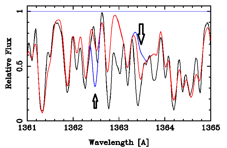
The smaller upward arrow gives the position of B II 1362.46 and the blue line shows the profile if boron had a solar abundance. To prevent the boron feature from absorbing below the observed spectrum, we used a boron abundance decreased by 1.8 dex, or a factor of about 60. Given the complexity of this region of the spectrum, this is satisfactory agreement with JDL's assessmant that boron is "...about a factor of 30 times lower than the solar abundance..."
Our oscillator strength for the B II line is from Morton, D. C. ApJS, 149, 205 (2003). `
The Cl I line at 1389.96 also leads to a solar abundance for chlorine.
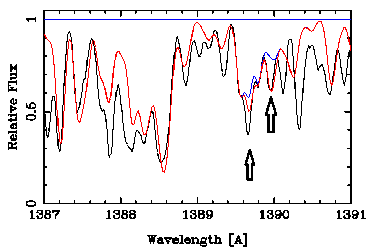
One can also see some absorption from Cl I 1389.69. The blue line shows the calculation with no chlorine.
Oscillator strengths for Cl I are from Chang, et al. J. Phys. Chem. A 114, 13388 (2010).
See the discussion for boron for an explanation of the line at 1362.46A. JDL reported [Cl/H] = -6.70 with an uncertainty of 0.3 dex. The solar [Cl/H], is which we find from 1363.45 is -6.54.
A fit with the log(gf) = -0.177 from the NIST Handbook yields an abundance excess of about 0.3 dex. This line was included in the study by Takeda, et al. PASJ, 64, 38 (2012), who give a NLTE correction of about -0.3 dex. Thus, our value is essentially solar, in good agreement with Takeda, et al.
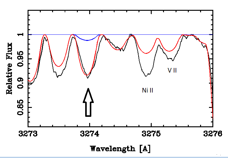
The blue line shows the calculation with a solar Cu abundance, the red with an abundance excess of 1.0 dex. A new calculation of the oscillator strength for Cu 3274 by Liu, et al. (2014, ApJS, 211, 30) is in excellent agreement with the VALD3 value used here. The stellar spectrum is from the UVESPOP archive, courtesy of S. Bagnulo.
Note the two underpredicted features due mostly to Ni II and V II.
We adopt a +1.0 dex excess for copper.
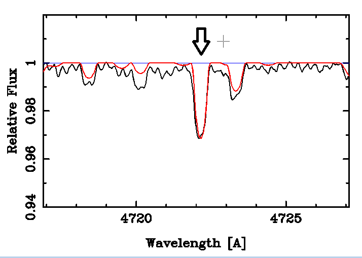
The resonance lines of Zn II, at 2025.48 and 2062.00. Both lines are significant contributors to their blends. Rather nice fits are obtained, as shown for the line at 2062A.
However, the zinc abundance required for the fit shown has only an excess of 0.25 dex above solar. A comparably nice fit for the line at 2025 requires an excess of 0.65 dex. Thus both Zn II lines disagree with one another and with the three Zn I lines, which are in good agreement. The oscillator strengths for Zn I are due to Biemont and Godefroid (1980, AA, 84 361). They are in excellent agreement with a more recent calculation by Liu, et al. (A&A, 536, A51, 2011). Though somewhat old, they are still used for the solar zinc abundance (Grevesse, et al. 2015, AA, 573, 27), and should certainly be reliable to within 0.1 dex (or better). The Zn II gf-values were recently calculated by Kisielius, et al. arXiv: 1504.01667, who obtained values within 0.1 dex of those from VALD3. We suggest the problem is with the blending of the stronger lines.
We adopt a zinc excess of 1 dex.
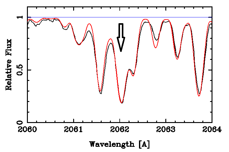
There is a good account of gallium in stellar spectra in the Jaschek's 1995 book The Behavior of the Chemiscl Elements in Stars, Cambridge Univ. Press. In Sirius, we looked only for the Ga II resonance line at 1414.40A. There is a strong feature at this position, but it is clearly a blend of a number of lines. The case that Ga II is a strong contributor to the blend is made in the following figure.
The blue line shows the synthetic spectrum with gallium set at the solar abundance, while the dashed blue line was computed with no Ga at all. Clearly a major part of the absorpton on the red side of the blend is due to Ga. The strong absorption on the violet side of the blend was measured separately at 1414.312, and is primarily Fe II and Ni II. The oscillator strength of the Fe II line was increased to fit the violet side of the blend. The red spectrum was calculated with gallium enhanced by 0.07 dex.
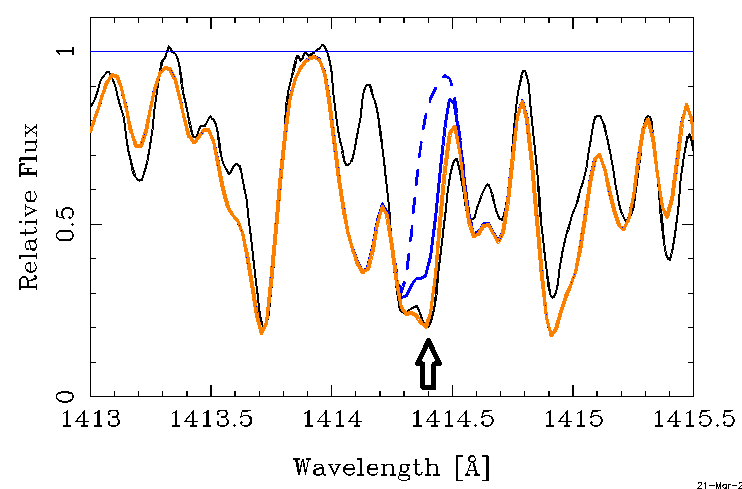
Consistent upper limits were obtained from three Ga I lines from the ground term, at 2041.71, 2068.66, and 2094.26. Oscillator strengths were from Morton's (2000) compilation. In the case of all three lines, an abundance excess of 2 dex caused unobserved absorption, while an excess of 1 dex was compatible with the observed spectrum.
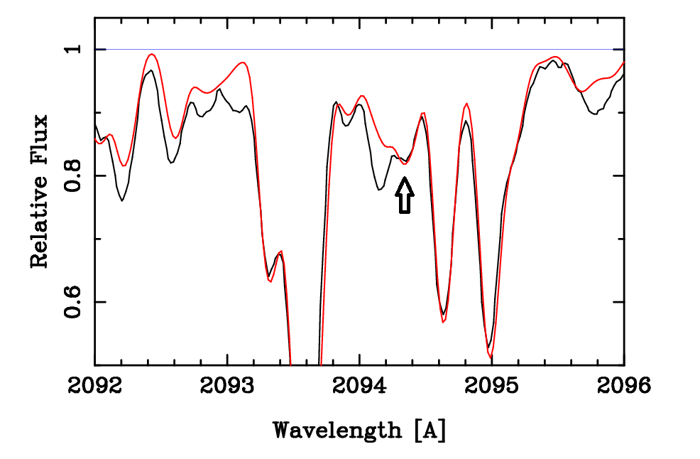
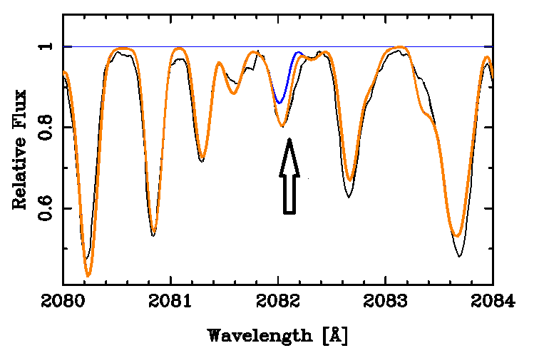
The figure shows the a feature at the wavelength of the Ge I line 2094.26, where the abundance has been increased until the feature is clearly overpredicted (too strong). We adopt a slightly smaller germanium abundance as our upper limit. It agrees with the observed spectrum--with an abundance enhanced by 1.3 dex over the solar value.
A substantial fraction of the absorption in the violet portion of a strong blend near 1649.5 is due to Ge II 1649.19. This is shown in the figure, where the blue line indicates a calculation with germanium omitted.
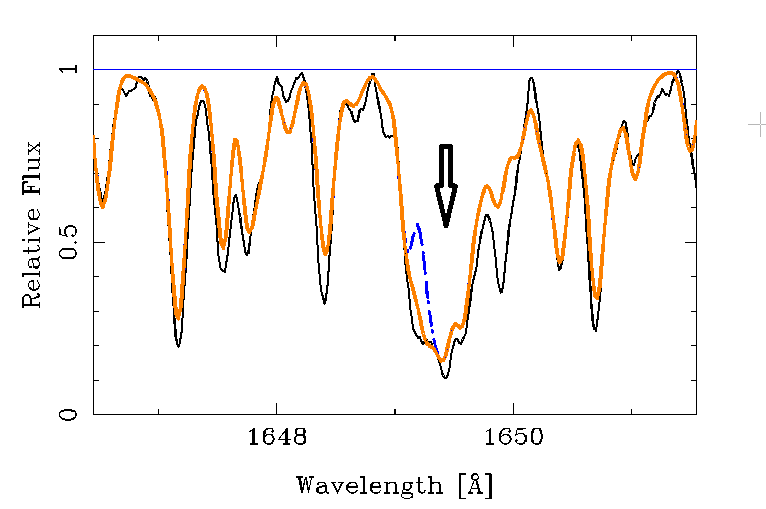
Using the oscillator strength from NIST, due to Fuhr and Wiese (2005, Handbook of Chemistry and Physics, 86th ed), we require a slightly sub solar germanium abundance (-0.29 dex). This could indicate an even-Z anomaly. The Ge II line comes from the dominant ion, but the accuracy of the log(gf) was unassigned by NIST. Moreover, the blend is significant. Overall, we assign the germanium abundance to be +0.5 dex, with an uncertainty of surely 0.7 dex.
The As II lines are not favorably placed. As I has possibly been identified in some stars. Since the first ionization energy is 9.8eV, we synthesized a region around the strong As I line at 1890.42A. We used an oscillator strength from Gans, AAS, 143, 491 (2000).
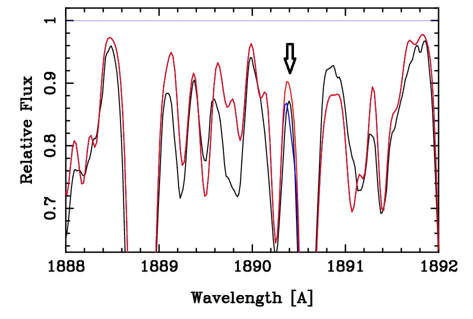
The red line indicates an arsenic enhancement of 0.8 dex, while the blue was made with 1.3 dex.
Synthesis near the As I line at 1972.62 is shown in the figure below.
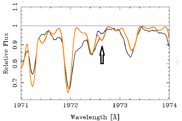
Note that the VALD As I lines need attention. By chance, we noted that the Al I line 1936.46 has much too large a gf value (+0.602). Kurucz gives -0.303 (gfemq1300.pos).
A fit is shown in the figure (arrow), using solar abundance (blue), and an enhanced selium abundance. Spoiler Alert: The observations are near the limit of the vacuum wavelengths, and the resolution of the observations is clearly inferior to that at shorter (and longer) wavelengths. We therefore suspect some problems with the adjustment of the observations, and have shifted them by about 0.01A to obtain better agreement with the Se I profile. If we accept that shift, the fit (red) corresponds to an enhancement of selenium of 0.76 dex. Without the shift, the fit, the minima of the calculation and observation do not fit well, and an upper limit of about +0.5 is obtained. This conclusion is perhaps the most prudent.
The oscillator strength is from Morton, ApJSuppl., 130, 403 (2000).
We conclude that the bromine abundance in Sirius is 1.4 dex above solar.
The plot shows a calculation with krypton +3 dex (red), and +4 dex (blue) overabundant. The observation is from a UVES spectrogram, but the placement of the continuum is uncertain. Nevertheless, from this line, it not realistic to place an upper limit to the krypton abundance lower than 3 dex above solar.
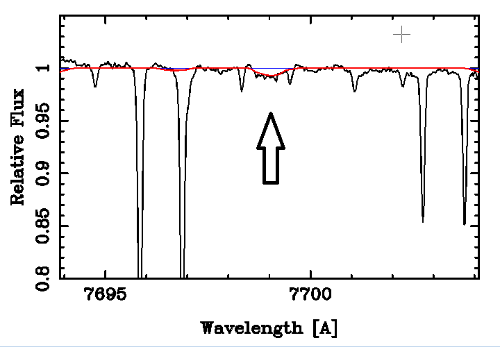
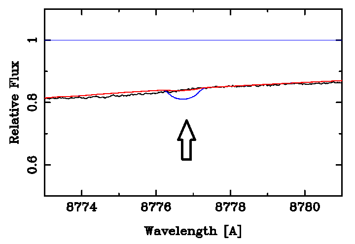
A slightly lower upper limit was obtained from the Rb I resonance lines at 7800.27 and 7947.60. A synthesis of the second of these is shown.
The blue line represents a calculation with no Rb at all, and the red was made with an excess of +2.7 dex. In principle, an upper limit from this line could be found by reducing the Rb abundance until no trace of the blue line could be detected--even with a magnifying glass. That abundance corresponded to a 1.26 dex excess. However, the difference between this and a 1.7 excess was hardly discernable. We adopt an upper limit of 1.7 dex.
A Nb II line at 2697.06 is relatively shallow. The stellar feature was measured at 2697.03, with a central intensity of 0.89. Depending on the placement of the continuum, the feature is partially or totally accounted for by Co II 2697.04. The following figure shows a relatively wide region surrounding this line, so one can judge whether the continuum is properly placed. If one assumes that placement and the relevant oscillstor strengths are correct, much of the absorption is not accounted for by the Co II line.
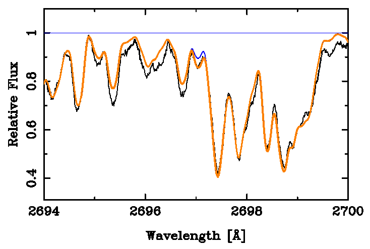
In the figure, the position of the Nb II line is marked with an arrow. The blue line was calculated assuming a solar Nb aundance, while the red line, which is a close fit, assumes a Nb abundance enhanced by 2 dex. The other Nb II lines make us skeptical of a full 2 dex excess of Nb. However, a 1 dex, or slightly larger enhancement is plausible.
Several lines from Multiplet 1 of Nb I are north of optimum STIS coverage. The figure shows a synthesis near 3215.60.
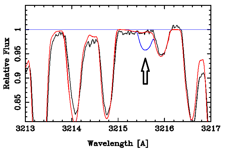
The blue line is made with a niobium excess of 2 dex above solar. It is clearly ruled out. The red line uses a 1 dex excess over solar, and is an upper limit. The red line cannot be distinguished from one using solar niobium.
Two lines just north of the STIS coverage, may be found on the COPERNICUS spectrum. Ths STIS spectrum in this region is noisy. The lines are at 3094.18 and 3130.79A. Both regions may be satisfactorily synthesized with solar abundances of Nb. However, equally good fits may be obtained when Nb is increases in abundance by 1 dex. A 2 dex increase, however, leads to absorption that is not observed.
A similar remark holds for Nb II 2033.01 (log(gf)=+0.33) and 2109.43 (log(gf) = +0.25). Both oscillator strengths were interpolated using the MCS intensities and three lines for which gf-values were available from Nilsson, et al (2010). We can clearly rule out an excess of 2 dex, and a 1.5 dex excess also overfills the observed spectrum. But an excess of 1 dex is hardly distinguishable from no Nb at all.
We adopt an upper limit of 1 dex.
There were 29 Mo II lines in the >2000 list, but only 9 had "plus" depths > 0.1.
A WCS run looking for 34 Mo II lines gave no significance. The stronger
persistant NIST lines are
wavelength    I       CI   STIS-wl    ID1     dep    ID2       dep
2015.109      500                                                     No line measured near this wl
2020.314     1000    .78  2020.303  .31 Mo II .645; .33 Cr II .596  Sadakane synthesized this line
2038.452      500    .85  2038.465  .42 Cr II .148  .45 Mo II .386
2045.973      400    .83  2045.933  .91 Cr II .742  .97 Mo II .377
The feature near 2020.31, has an equivalent width of about 40mA. It was identified as Mo II by Sadakane (1991, hensforth, KS), who showed that other known contributors could not account for the observed amount of absorption. From synthesis, we also conclude that this feature is primarily due to Mo, with small amounts of absorption, not more than about 10\% from known lines, due mostly to Mn II. We have computed an abundance using log(gf) from NIST based on Silkstrom, C. M., Pihlemark, H., Litzen, U., Johansson, S. Li, Z. S. \& Lundberg, 2001, J. Phys. B, 34, 477. They give \log(gf) = 0.022. The result is dependent on the assumed microturbulence (ca. 2.0\kms), as well as the resolving power relevant to our spectrum (ca. 13 500). The synthesis is shown below. The blue line shows synthesis assuming solar molybdenum.
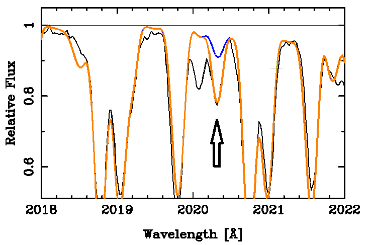
Our best estimate from this line is Mo/Ntot = 0.6E-09 or log(Mo/Ntot) = -9.2. This corresponds to [Mo/H] = 0.93.
We synthesized the regions around the three strong, zero-volt Ti II lines at 2543.23, 2609.99, and 2647.01A. Oscillator strengths are from Palmeri, et al. MNRAS, 374, 63, 2007. A more recent study by Zhang, et al. A&A, 551, 136 (2013) does not contain these lines!
We took as a default abundance Tc/(Ntotal)= 0.248E-10, which is the same as the solar Nb abundance. In the plot below, the blue line assumes tecnetium has an abundance 1 dex above the default value. The red calculation was made assuming no tecnetium at all!
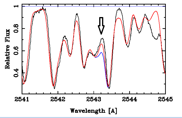
Because the spectrum at 2543.2A is overpredicted, even with no technetium, we must conclude that the abundances and/or oscillator strengths of other species near this wavelength are overestimated. Overprediction of absorption is common, as a scan through our figures will show. This might lead us to believe that underestimates of abundances would be common. This has not been the case.
Some of the lines in this region in VALD3 appear to be pairs that are the same line but with slightly different wavelengths from different sources. Other Guesses need to be updated with Palmeri, et al. 2009.
The line at 1875.56A, while closely blended with the Fe II line at 1875.53, is the best case for the presence of Ru II in the STIS region. The calculated profile at the position of the line is weaker than the observed one. Palmeri et al. J. Phys. B, 42, 165005 (2009) give log(gf) = -0.23.
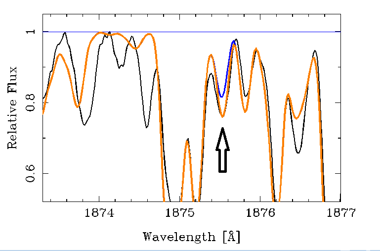
In the figure, the arrow marks the position of the Ru II line, and the blue was made assuming no ruthenium at all. A solar abundance of of ruthenium hardly changes the calculation from the blue line. That is because of a relatively strong Fe II line at 1875.53. VALD3 gives the source of the log(gf) for Fe II as K13 (Kurucz 2013). We find no other source for that line. If we use the default log(gf)'s for the Fe II and Ru II, the ruthenium abundance that fits (red line) has an excess of 1.2 dex.
Kohl (1964) has several lines identified as blended Ru II. We looked at the region near 3221, where Kohl has Ru II-3 3221.38 and Ru II-7 3221.98 (He gave 49mA, however, our nearest measurement was 3222.06.). These weak features cannot be Ru, as they require an enhancement of over 3 dex, which can be ruled out. Recent oscillator strengths are from Palmeri, et al. (2009, J. Phys. B, 42, 165005).
The figure below shows a region with two Ru II lines, 1939.04, and 1939.51. Only the second of these has a nearby measurement (1939.54), but it is plausibly attributed to Fe II, at 1939.55A.
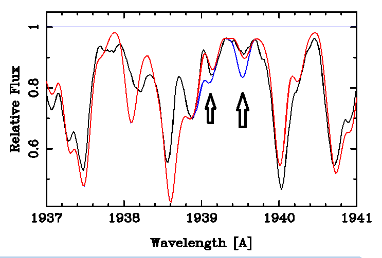
The blue line shows the result of a 2 dex enhancement, while the red is for an enhancement of 1 dex. The plot is unchanged if we reduce the ruthenium abundance to the solar value.
A Cr II line in VALD3 and on Kurucz's (11 April 2015) gf2401.pos at 1939.301A does not appear in the NIST list of Cr II wavelengths. It was predicted by Castelli (web site) for HD 7143, but is not in the stellar spectrum. The transition, 3d6 4s2 4D1.5 -- 3d3(4F)4s4p(1P)4D^o1.5 is a difficult calculation. We have reduced its already small log(gf) by 1 dex.
We also looked at the close pair Ru II 1966.07 and 1966.73, shown in the figure below.
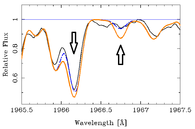
In the above plot, the blue line is made with a solar Ruthenium abundance. However, the plot is hardly changed if the abundance is assumed to be +1.0 dex. Given the undertainties, we cannot rule this excess out. The brown line is made with an assumed excess of 2.0 dex, which surely is excluded.
We adopt a +1.0 dex as an estimate for the ruthenium abundance.
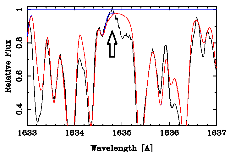
The figure shows a region around Rh II 1634.72, which has a relatively new oscillator strength from Quinnet, et al. A&A, 537, A74 (2012), and Bachstrom, et al., J Phys. B., 46, 205001 (2013). There is a (noisy-looking) local maximum of the stellar spectrum near the Rh II position. The blue calculation is for a rhodium excess of 1 dex, while the red is for a 2 dex excess.
A second line with a new oscillator strength, at 1637.88, is unusable because a calculated V II line at 1637.95A overfills the observed spectrum.
Regions near lines of Rh II at 2415.84 and 2420.97A were synthesized. That near the former is shown.
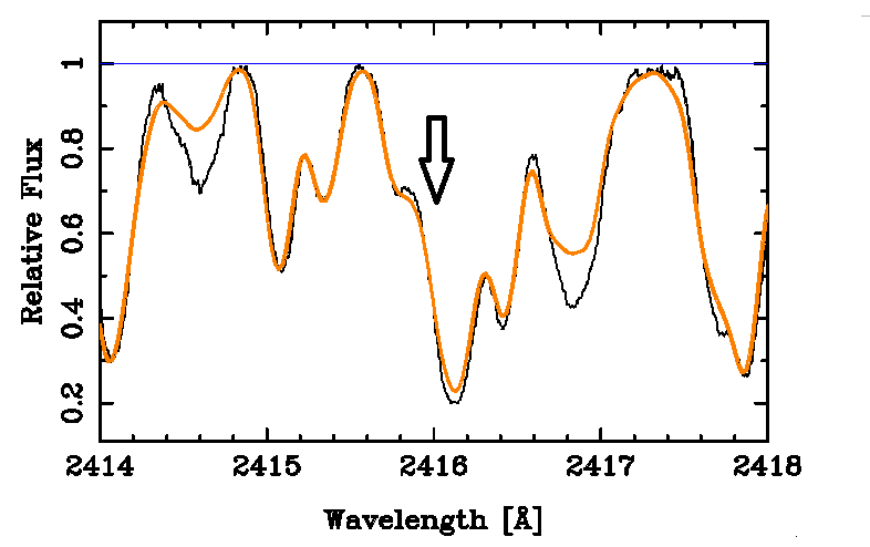
We estimate an upper limit for rhodium of +1.5 dex.
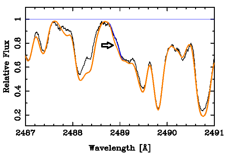
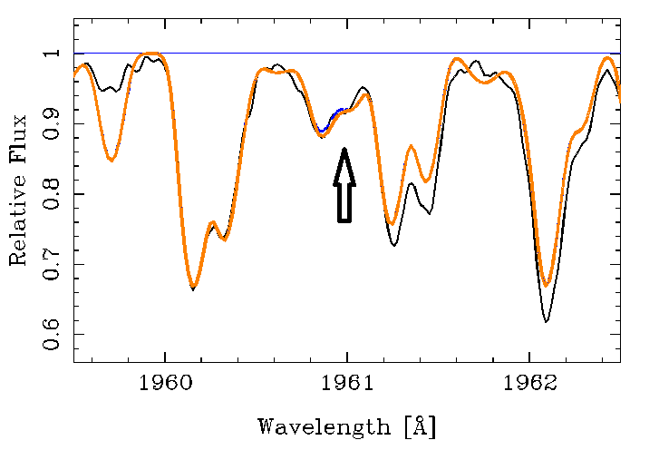
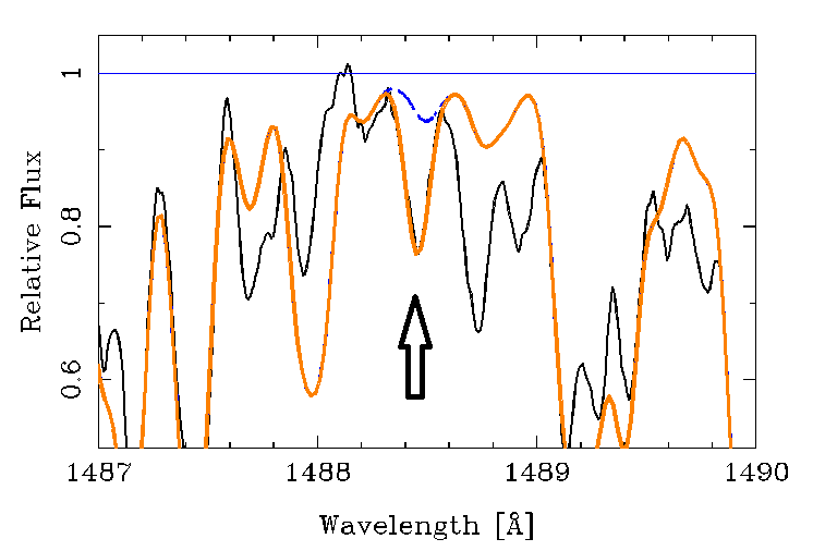
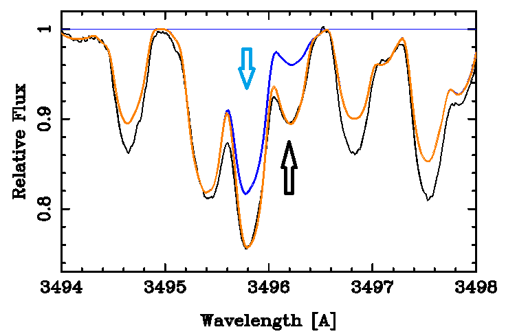
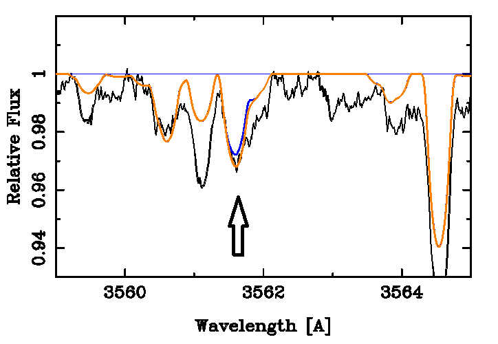
The plot shows synthesis near Pd II 2488.91. As usual, observations are in black, and a calculation in orange assuming an enhancement of 2 dex over solar for palladium. The wide blue line shows the calculation with no palladium at all. For most of the calculation, the orange and wide blue coincide, and the enhanced palladium shows up only near the position of the horizontal arrow. The observation and calculation with no palladium coincide where the blue line has no orange component. The orange differs from the blue because it was computed assuming a +2 dex enhancement of palladium. It is difficult to display, but we discern a difference between the observation (which also coincides with no palladium, where the arrow points), and a palladium excess of 1.5 dex
On the basis of this calculation, we adopt an upper limit for palladium of 1.5 dex over the solar abundance.
Palladium was not identified by YG.
The VALD3 wavelengths do not agree with current NIST postings, and should be replaced. We use the NIST source from Kalus, et al. Phys. Scr. 65, 46 (2002). Transition probabilities are from Biemont, et al. J. Phys. B 30, 2067 (1997). In the figure, we show a calculation of the region near the Ag II line at 2246.41A, which has an A-rated transition probability (1-3% error). The line falls at a relative high of the spectrum, where no minimum is obvious. Since the abundance or upper limit estimate depends critically on the placement of the continuum, a synthesis was made of the 40A-wide region shown.
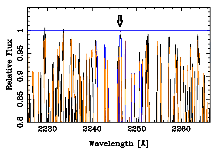
One can see that if the continuum were chosen on the basis of the high points near 2230A, it would be higher than the apparent local continuum near 2246A. Ultimately, we lowered the continuum estimate by 1% from the value shown in the wide plot, as shown below.
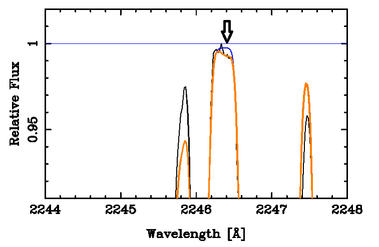
The calculation in orange (brown) shown was made with Ag/Sum = 0.100E-09. The blue shows a calculation with the solar silver abundance. The continuum choice is admitedly subjective. The calculation here corresponds to a silver abundance of 0.100E-9, which we adopt as an upper limit for silver. It corresponds to an excess over the solar value of +1.1 dex.
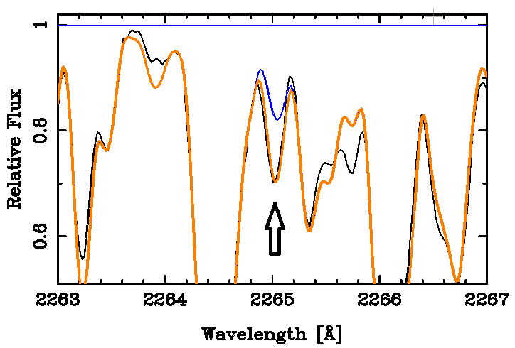
The 2265 line of Cd II is the weaker of an s-p resonance doublet. We get a good fit to the feature (orange line) with Cd/Ntot = 0.270E-09, or an excess over the solar value of 0.7 dex. This is somewhat smaller than the value calculated by KS, but his fit did not include the Fe I line at 2265.05.
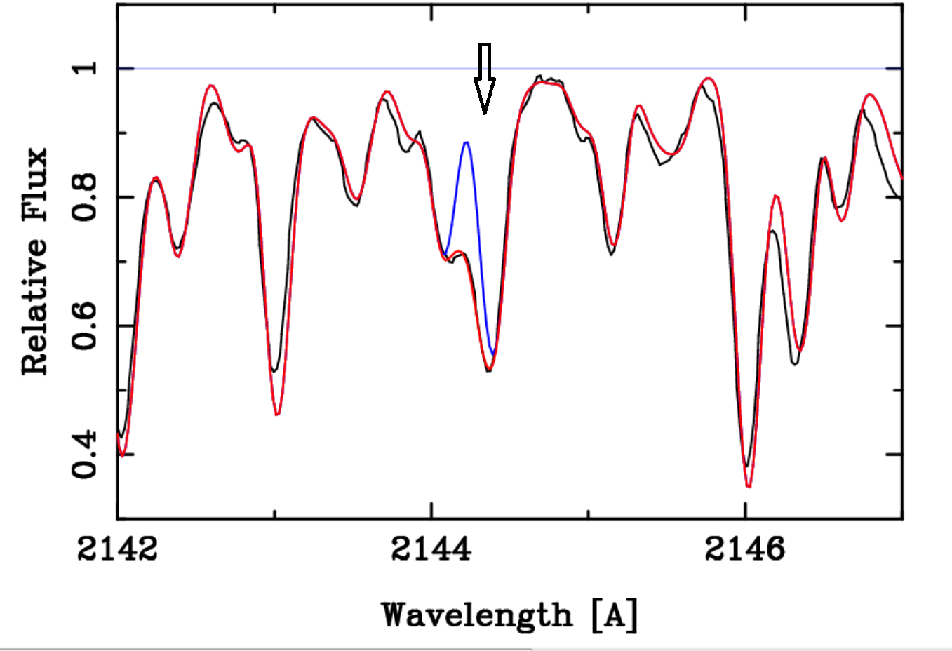
The Cd II line as 2144.41 makes a significant contribution to the feature measured at 2144.366, which is also blended with Pt II 2144.25. and also Cr II 2144.08. This blend is discussed in more detail below. It cannot be explained without contributions from both cadmium, platinum, and Cr II. The cadmium excess adopted on the basis of this line is 0.66 dex. This is shown in the figure below. The red line shows the calculation using both the cadmium and platinum adopted. The blue line shows the effect of using no cadmium at all.
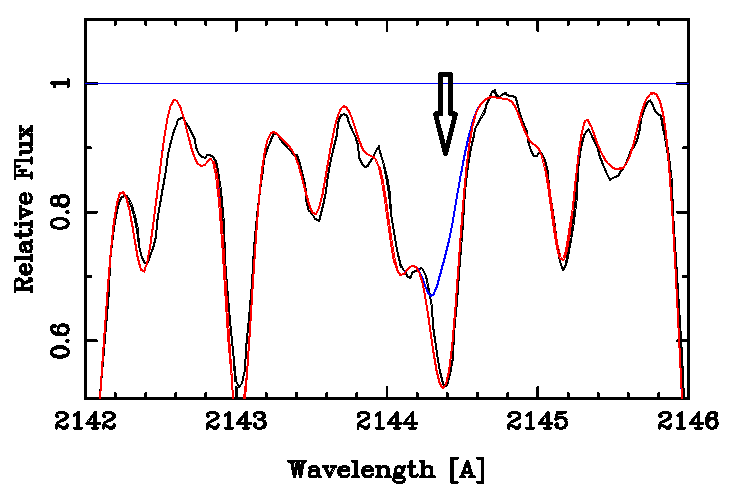
These identifications and excesses over the solar value for cadmium are expected for an element with this atomic number in a metallic line star. Oscillator strengths are from Glowacki and Migdalek, Phys. Rev. A. 80, 042505 (2009). We adopt an excess of 0.7 dex.
Neutral indium has an ionization energy of only 5.8 eV. Only one line is known in the solar spectrum, and its abundance is at odds with the CI values.
The most likely line of In II is the resonance line 5s2 1S -- 5s5p 1P^o at 1586.34. The wavelength and oscillator strength (log(gf) = 0.14) are updated from VALD3; see A. Kramida (J. Res. NIST,118, 52, 2013), and L. Curtis (Phys. Scr. 62, 31, 2000).
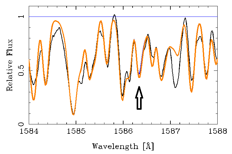
The Ritz wavelength has been corrected in Sansonetti, Martin, and Young (2005). We use their value, 1586.34A, which is essentially coincident with Fe II 1586.33. This wavelength differs by 0.03A from the Ritz value, which may be found in atomic data bases.
One can hardly see the blue (solar abundance) synthesis as it differs so little from the adopted (orange) synthesis. Therefore we show a blow up of just the region in question.
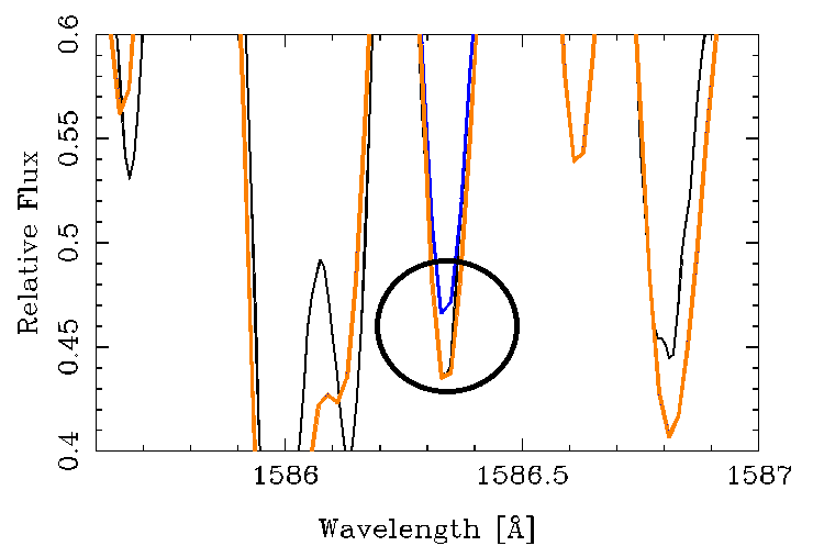
The fit to the observed minimum was made with an excess of 1.8 dex over the solar value, which we adopt as an upper limit. The uncertainty is at least 0.3 dex.
Tin was not among the elements reported by KS in the Copernicus spectrum, but it is listed among those found by YG. A WCS run using 7 of the stronger lines from the VALD3 prediction was not significant at +/- 0.06A, but at +/- 0.03A, the estimated probability that the 4 out of 7 lines found was 0.07. This is "just" below the usual threshold of significance (0.05), but in view of subsequent calculations, we do not dismiss this marginal result.
We synthesized the regions around 4 of the strongest Sn II lines. All are significantly blended. The abundance estimate is based on the line at 1899.90A, as shown below, with the solar abundance calculation shown in blue.
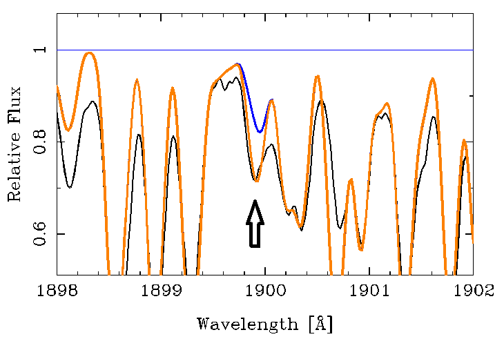
The Sn II oscillator strengths are graded B+ by Haris, et al., Phys. Scr., 89, 115403 (2014), so the "needed excesses" are attributed to unknown contributors. The stronger blend on the long wavelength side of the Sn II line was "modeled" The orange spectrum was made with an assumed Sn abundance of 4.5E-10, or an excess of +0.7 over the solar value.
There are no Sb II lines in VALD3 for the region of the STIS lines. There are Sb II oscillator strengths for two lines, at 1384.66, and 1436.45A in the NIST Handbook. However, these lines are not suitable, even for upper limits. The main problem is that the Sb II lines 1384.66 and 1436.45 are very closely blended with strong lines from Fe II, Cr II, and Mn II.
We found one line, at 1387.56 that did not correspond to a measurement, but was suitable for a crude estimate at an upper limit. However there was no published log(gf) for this line, so we calculated one with the Cowan code (log(gf) = -0.337). Prior to attempting the calculation, we set the antimony abundance to zero, and adjusted oscillator strengths of nearby lines to fit the observed region from roughly 1387.4 to 1387.8A.
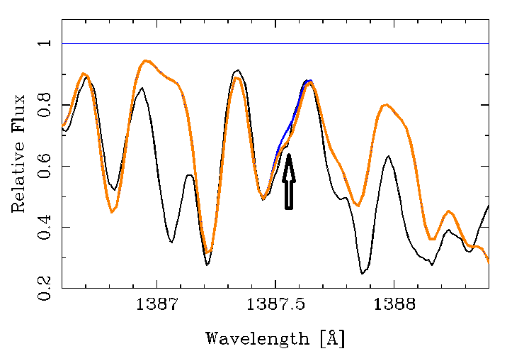
The blue line in the figure shows a calculation with the solar antimony abunance, which is not different from the profile with no antimony at all. The orange curve shows the result with the antimony abundance incresed by 1.3 dex. We adopt that as our upper limit.
The NIST Handbook lists three transitions of Te II from the ground level, all below 1300A. Some strong lines of Te II are in the visible, but are of quite high excitation. We looked at 4654.37, 5649.26, and 5708.12, on the FKW atlas, and found no clear indication of Te II. Oscillator strengths have only recently become available for Te II (Zhang, W., Paleeri, P., Quinet, P., and Biemont, E. 2013, A\&A, 136, 551).
We made a calculation for 1461.678, whose lower excitation is 2.55 eV.
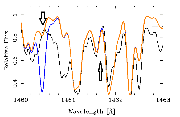
In the region of Te II 1461.68, the spectrum calculated with solar tellurium is hardly distinguishable from the orange curve that used an enhancement over the solar abundance of 1 dex. We adopt +1 as the upper limit for tellurium.
We are unaware of a robust astronomical detection of iodine in stellar spectra. Jaschek and Brandi (1976, A&A, 20,233) suggested that 4 lines attributable to I II had been found in the spectrum of HD 25354. This was one of the Ap stars studied by CRC and coworkers in the 1970's (Cowley, Aikman, and Hartoog 1976, ApJ, 206,196). With higher resolution material than that available to Jaschek and Brandi, we found no evidence of I II. A current search of wavelength measurements on 2 plates of HR 25354 does not support the I II identification in that star.
The resonance lines of the second spectrum of iodine are below 1250A and unusable in the present and most studies.
Neutral iodine has an ionization energy of 10.4 eV. Consequently, we used oscillator strengths from NIST to synthesize regions near the stronger zero-volt lines at 1702.07 and 1782.74. The first of these lines is overwhelmed by a strong Fe II line, 1702.04. In order to get noticable absorption from iodine, an abundance enhancement of some 4 dex was necessary. The 1782.74 feature is mostly due to P I, 1782.83. An iodine contribution to the absorption becomes noticable if the abundance excess is some 3 dex.
There is a strong I I line at 1830.38, but it is in a complex blend. We set the iodine abundance to zero, and modeled the feature by adjusting the gf-values of nearby lines until the observed absorption was closely fit. We then asked what iodine abundance would become marginally noticable. That value was somewhere in the excess of 2.4 to 2.7 dex above solar. This was our upper limit from the 1830 line. It is larger than the abundance estimate we obtain from the line at 1457.98A, which we now discuss.
The NIST Handbook lists a zero-volt line at 1457.98A. A transition probability was calculated by Chang, Kum and Dong (2010, J Phys Chem. A, 114, 13388). From their Table 3, we obtain log(gf) = +0.196. Interestingly, the "by eye measurement of the STIS spectrogram has a measurement at 1457.983. The strongest nearby blend is Cr II 1457.94, which is too far away in wavelength to account for the observed absorption. Synthesis of the region is shown in the figure.
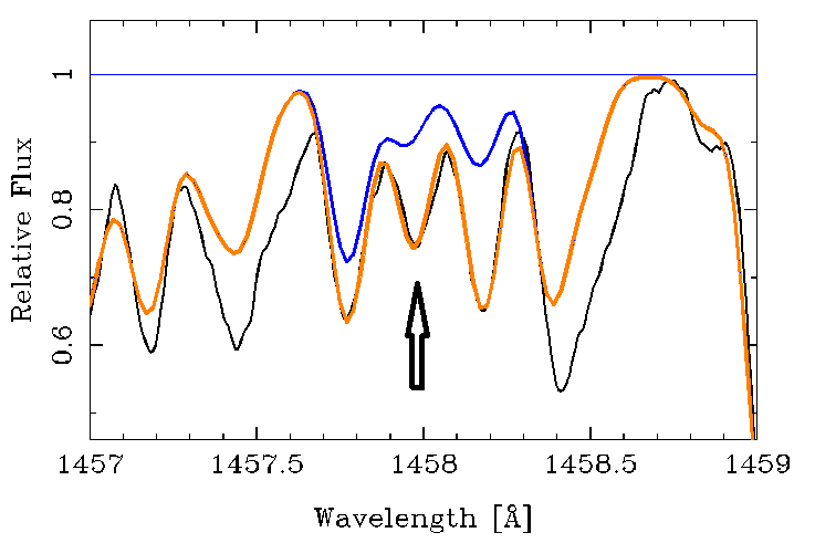
The blue line shows synthesis with solar iodine (black arrow). Oscillator strengths for Fe II lines at 1457.77 and 1458.19 were adjusted until their profiles fit the observed spectrum. That was done in case these lines made a contribution to the putative iodine absorption. The blue shows their absorption with default (VALD3) gf values. We also made a calculation using the full hfs for I I 1458 (12 components). Because the splitting is quite small, the computed spectrum hardly changes, though a slightly smaller (0.1 dex) abundance is needed for a fit. That excess, which we adopt is 2.1 dex. Given that many of the nearby absorption lines are underpredicted, it is reasonable to be skeptical that the iodine excess is a full 2.1 dex.
In looking for 1702.07, we found a nearby Be I line with a VALD3 log(gf) that apparently got a minus sign lost. They had log(gf)=+10.42, citing a 1974 paper by Laughlin and Victor. NIST gives log(gf) = -9.42, citing a 1999 paper by Tachiev and Frose-Fischer J. Phys. B, 32, 5805, 1999.
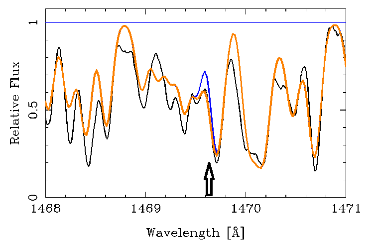
Only the violet wing of the Xe I line is perceptible. The main absorption is due to Fe II 1469.68 and Co II 1469.73. Nevertheless, xenon excesses exceeding 1.1 dex overfill the observed absorption on the violet. The stronger resonance Xe II lines also fall below our threshold of 1300A. Lines of Xe II are well known in the ground spectra of several peculiar A stars. Examples can be seen at the Castelli web site: http://wwwuser.oats.inaf.it/castelli/stars.html, we do not see any of these lines in the FKWW atlas. A calculation using the Xe II line at 5419.15A gives an upper limit of +3 dex. We adopt a xenon abundance 1.1 dex above the solar value, based on the 1469.61 line of neutral xenon.
Synthesis near the stronger of the Cs I resonance lines is shown in the figure. Ironically, there is an absorption quite near the 8521-line, but it is surely not due to Cs I.
We base an upper limit estimate on Ce II, 4603.79, shown below.
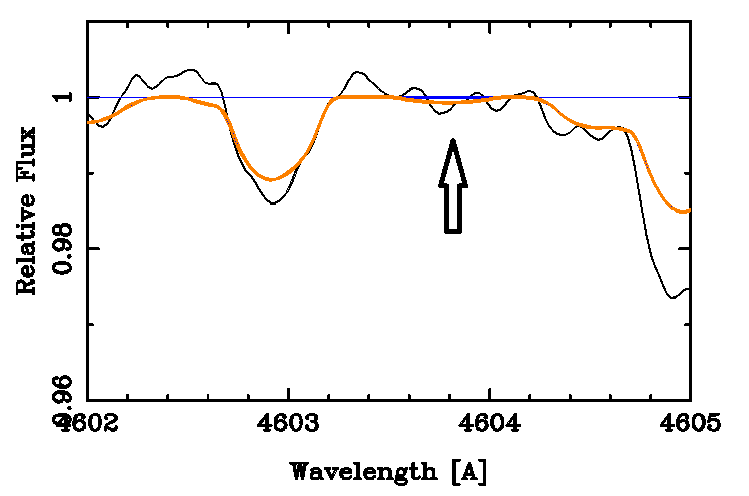
The second spectrum of cesium is xenon like, with resonance lines below 1000A. The lowest level of Ce II above ghe ground level has an excitation potential of 13.31eV. We found no oscillator strengths for the longer wavelength, strong Cs II lines. We made calculations using the strongest of the NIST Handbook persistent lines above 1000A, at 4603.79A. No feature was observed in the FWK spectrum. We base upper limits on an assumed log(gf) and a flat calculated spectrum. If we assume log(gf)=0.0, an absorption feature is marginally visible if the Cs excess over solar is 4.2 dex. We shall use 4.0 dex as our upper limit, with obvious caveats.
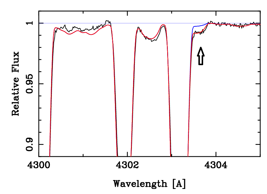
Little significant for lanthanum is to be gained from the STIS region. Qui, et al. give a lanthanum abundance based on a single line of La II at 4042.91A. They find log(La/H)= 1.88, which is about 0.84 dex above solar. If we use the Qui, et al. equivalent width of 8mA for 4202.91, our model, and a modern log(gf) value, we obtain an excess over solar of nearly 1.9 dex. Synthesis yields a poor fit to the profile shape, indicating that blends or perhaps hyperfine structure is relevant.
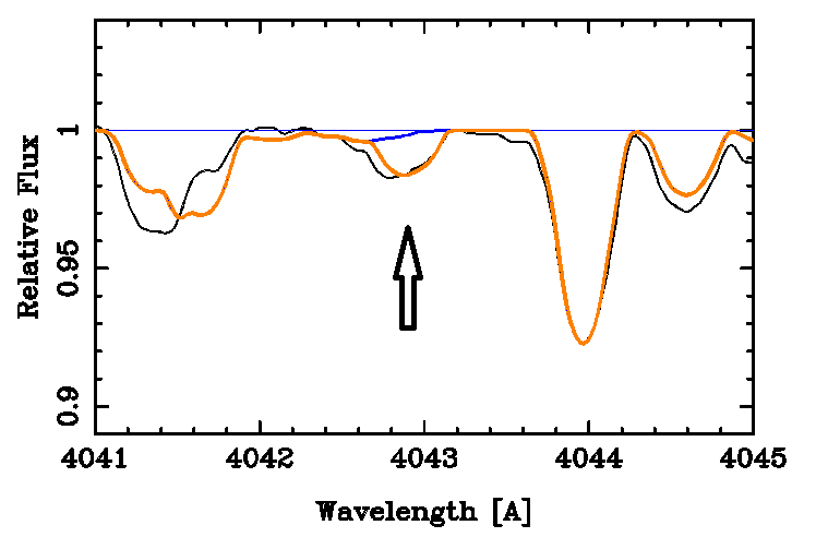
The figure shows the result of an assumed Lanthanum excess of 1.6 dex, which we adopt.
We found only 3 very weak Ce III lines in the UV and did not try to synthesize them. We adopt 1.5 dex for the cerium abundance excess.
Synthesis of a second Pr II line, at 4062.81 yields an upper limit of 2.3 dex.
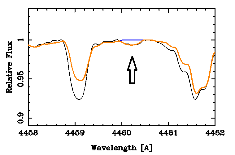
One of the strongest Pr III lines at 5299.99A is weak, but virtually unblended. The region is synthesized below.
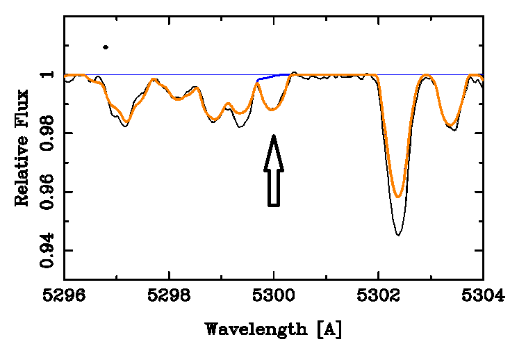
The best fit for the Pr III line is achieved with a praseodymium enhancement of 2.1 dex. The VALD3 oscillator strength used for the Pr II lines are from Biemmont, et al. European Phys. Journ. D, 27, 33 (2003). The VALD3 oscillator strength for Pr III 5299.99 cited as a private communication from A. N. Ryabtsev.
We find no indication of the abundance discrepancy between the second and third spectra from these three lines. Such a discrepancy is found in the magnetic Ap stars (Ryabchikova, T. 2014, in Putting A. Stars into Context, ed. Mathys, Griffin, Kochukhov, Monier, and Wahlgren, p. 220)
We adopt an excess of 2. dex for praseodymium.
We get another estimate from the mostly unblended line of Nd III, at 5294.10A. The synthesis is shown below. The large arrow marks the Nd III line.
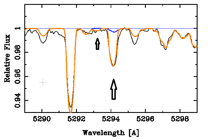
The oscillator strength is from Ryabchikova, et al. (2006), and yields an excess of 1.7 dex above the solar abundance. A moderately strong Nd II line, 5293.17, is nearby, and is fit reasonably well by the same abundance.
The lines are in good agreement with one another, giving an excess of 1.7 dex, which we adopt.
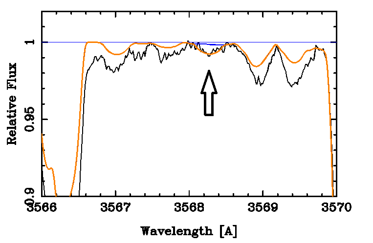
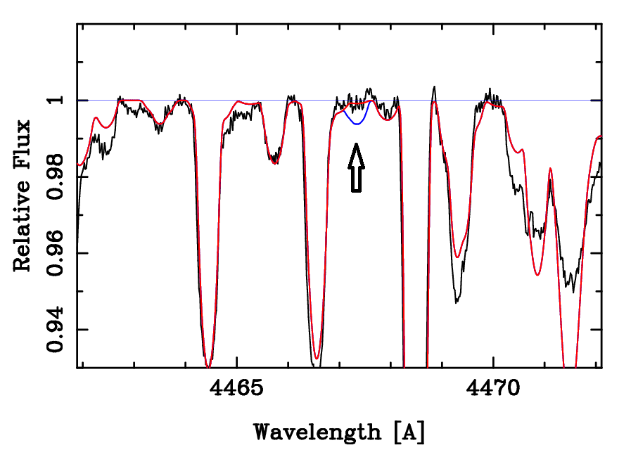
The Sm II line, at 4467.34 falls at a wavelength where there is very little absorption. The figure shows in blue, a synthesis using an excess of 2 dex, and is clearly ruled out. The red shows an excess of 1 dex, which we judge cannot be ruled out, and therefore take as an upper limit, based on this one line. The oscillator strength is from Lawler, et al. 2006, and is reliable.
If the continuum of the above plot were raised by 1 or 2%, the result from 4467 (ca. +1 dex) might be reconciled with those from 3568 and 3592 (ca. +2.3 dex). Clearly this element needs a more detailed study. We shall adopt +2. dex as a (provisional) upper limit for Sm.
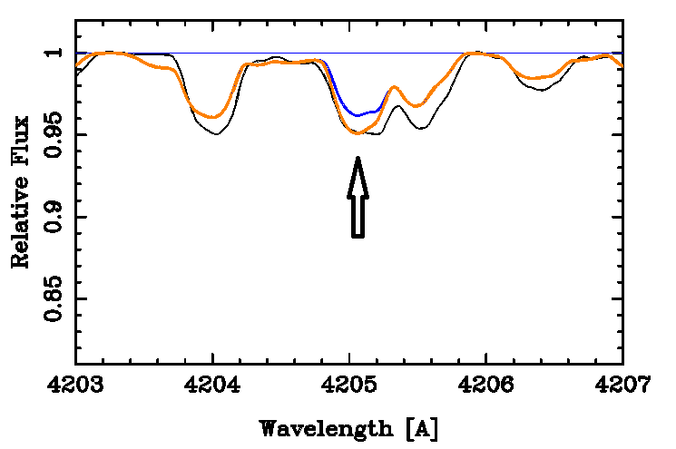
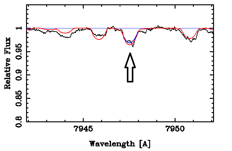
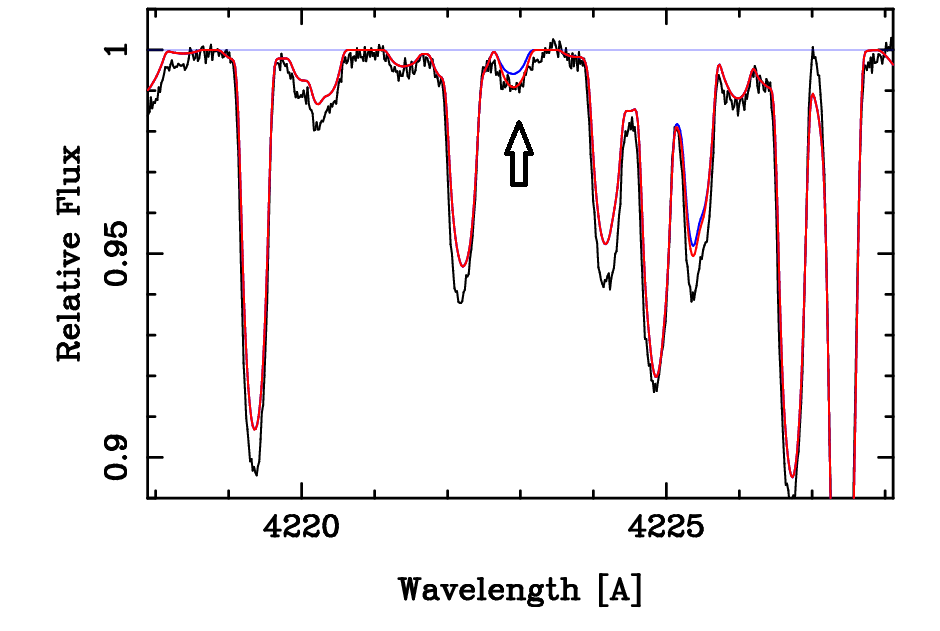
The blue line was made with a solar europium abundance, while the red was made assuming an enhancement by 1.5 dex. The Eu II is closely blended with two V II lines at 4205.04 and 4205.08. The Eu II line is a blend of Eu-151 and Eu-153 with the gf-values adjusted for a solar isotopic mixture. However, the full hfs has not been used.
We looked at 4 strong Eu III lines, at 2375.46, 2444.38, 2445.99, and 2513.76A. None were suitable for a good estimate. The region near 2513.76A afforded an upper limit of +2dex.
We adopt +1.5 dex for Eu.
Kohl (1964a,b) identifies a dozen or so features as Gd II. Almost every feature we looked at had problems. We analyzed Gd II lines at 3545.80 and 3549.36. We show the latter below.
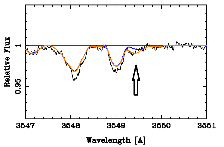
The blue line is with a solar Gd abundance, while the orange was made assuming a 1.5 dex excess. There is a high near the line center that we assume is noise. A compromise fit of the red wing of a line near Gd II 3545.80 gives a 1.4 dex excess, but with perhaps 0.2 dex uncertainty.
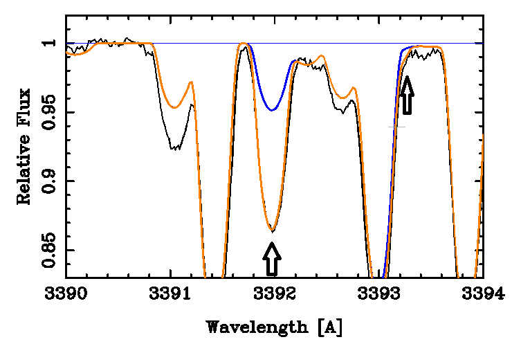
A Gd II line at 4251.73 overlaps with Mn II 4251.72. Default Mn II abundnce and gf-values are not sufficient to account for the abserved absorption. However, if we assume the Gd line causes the remaining absorption, we overfill two weak Gd lines at 4253.36 and 4253.66. Indeed, the latter two lines would be well fit by a solar Gd abundance! In the figure below, neither of the two regions indicated by the arrows is well fit.
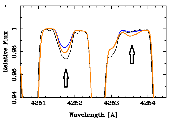
In the above figure, the blue line indicates a solar Gd abundance. The orange line assumes a Gd excess of 1.5 dex, and is a compromise between the two regions--one is underfilled and the other overfilled. Oscillator strengths for Gd II are from Den Hartog, et al., ApJS, 167, 292 (2006).
VALD3 had predicted 3 possible Gd III lines. The strongest of these was at 2223.95A. The figure shows synthesis in the region of this line.
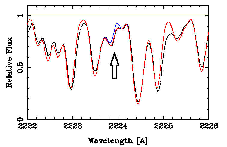
An absorption at 2223.84, mostly due to Fe II, was over predicted. We removed Gd entirely, and adjusted the log(gf) value of this line until the Fe II no longer overfilled the absorption. The result is shown by the blue line. A gadolinium enhancement of 1.65 dex is shown by the red line. This is a plausible result, but hardly a firmly established one. The oscillator strength for Gd III is from Biemont, et al. (2002, A&A, 393,717).
We adopt the +1.6 dex enhancement for Gd.
VALD3 has some KP Mg I loggf's at 2564.93 that are badly in error. Better values are at the Kurucz site.
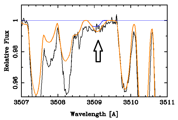
The obvious blending line, V II 3509.023, might well account for the entire feature if its oscillator strength were increased by 0.23dex. The terbium oscillator strength is by Lawler, et al. (ApJS, 137, 341, 2001). Certainly a terbium enhancement greater than 2 dex is ruled out. Thus 2 dex is our upper limit.
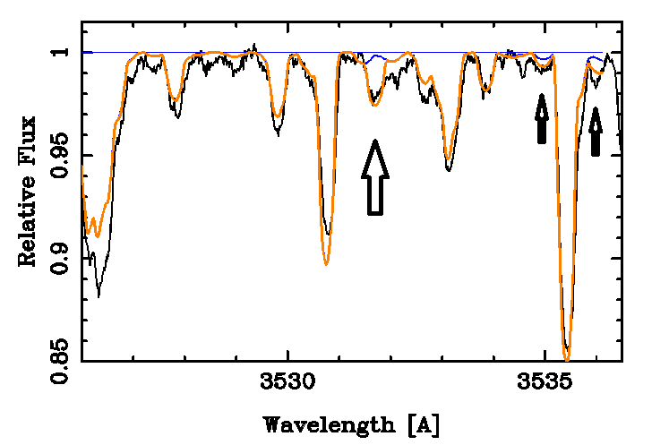
The blue line shows solar, while the orange assumes an excess of 1.7 dex above the solar value. The 3531.70 line is slightly overfilled by the calculation, while the two weaker features are slightly underfilled. We adopt 1.7 dex for the Dy excess.
Observed spectrum is from the UVESPOP archive, courtesy of Stefano Bagnulo. The blue line is for a calculation with solar abundance, while the orange was with an enhancement of 1.8 dex. An upper limit of +1.8 dex is appropriate for holmium.
The orange line uses an enhancement of +1.76 dex. We adopt +1.8 dex for the erbium excess over the solar value.
The observed spectrum (black) is from the UVESPOP archive courtesy of Stefano Bagnulo. Zero volt lines at 3131.26, 3462.20,3701.36, and 3761.33. A calculation based on weak absorption at 3462.20 shows the solar Tm in blue and an excess of 2.1 dex in orange.
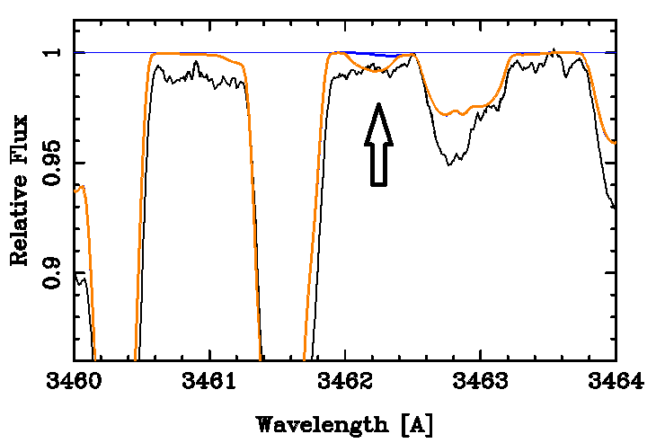
We adopt 2.1 dex as an upper limit for the Tm abundance.
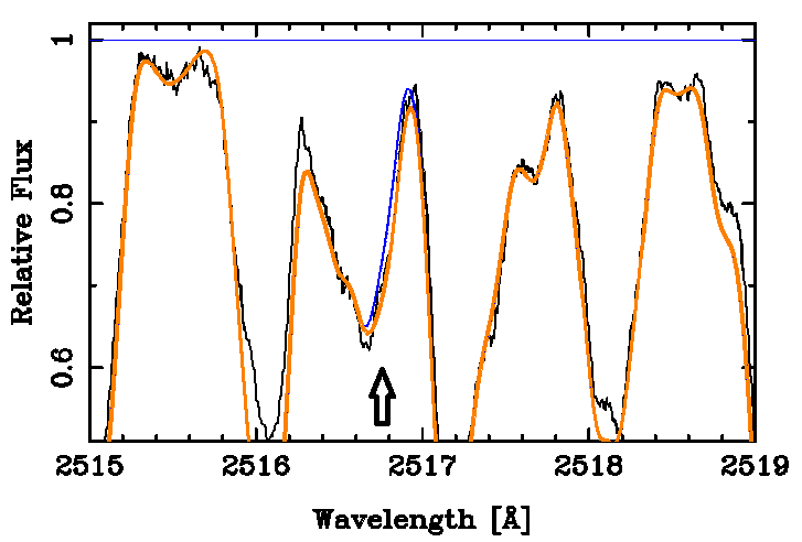
The blue line shows a calculation whith solar yttrium while the orange line was made with a 2.2 dex overabundance. The oscillator strength of Cr II 2516.55 was increased slightly to fit the violet wing of the blend.
The Yb II line at 3289.37A admits a lower upper limit. The figure again shows the synthesis with solar abundance (blue), and a +1.8 dex excess (orange). The Sirius spectrum is from the UVESPOP archive, courtesy of Stefano Bagnulo.
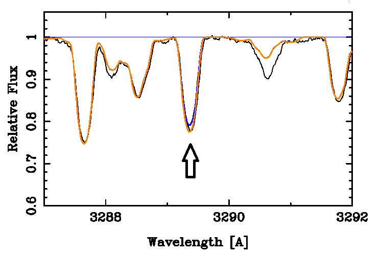
The Yb II line is virtually coincident with Fe II 3289.35.
We adpopt 1.8 dex as an upper limit.
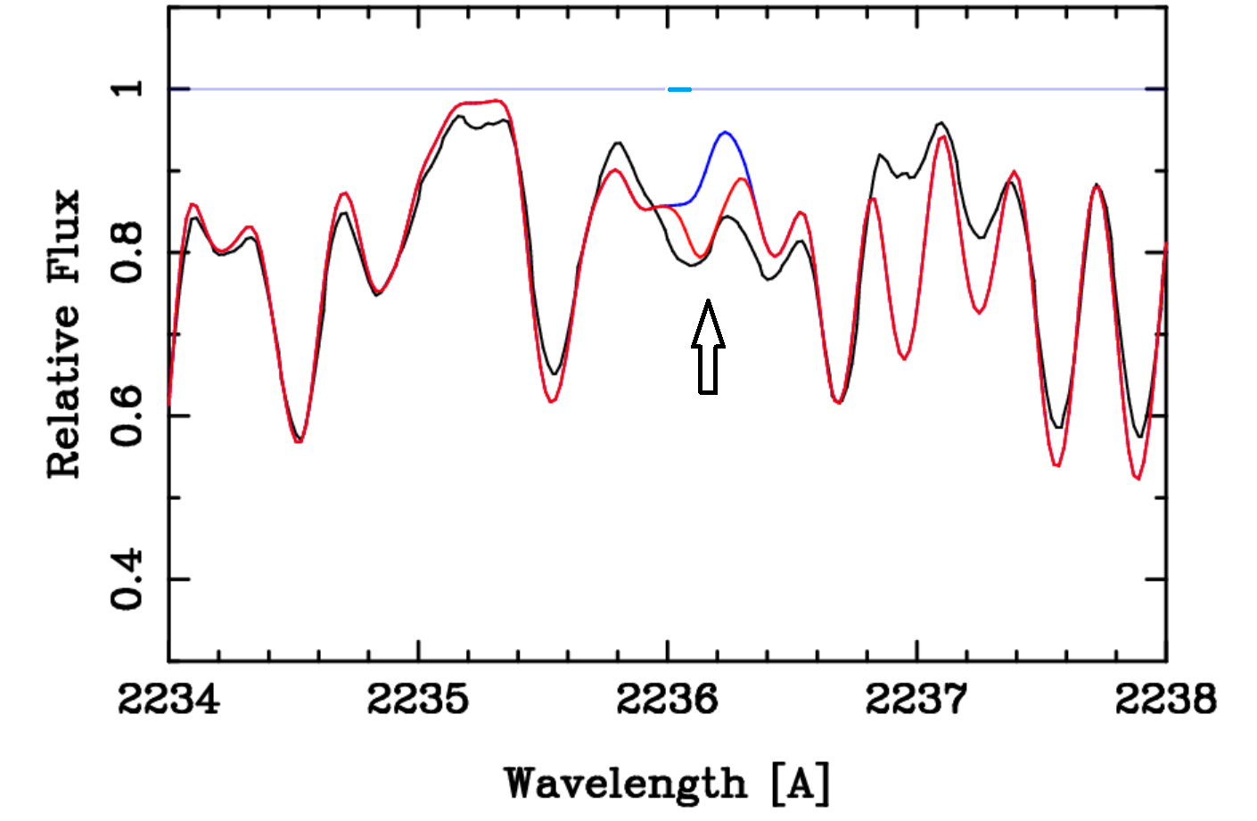
There is a strong line of Lu III at 2236.18A. The oscillator strength is from Quinet, et al. MNRAS, 307, 934 (1999). The region was synthesized assuming a solar abundance of Lu (blue), and an enhancement of 2.1 dex (red).
The region of another Lu III line, at 2603.35A, was synthesized.
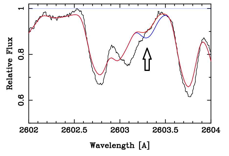
The red line shows a calculation with lutetium enhanced by 1 dex, while the blue shows the effect of an enhancement of 2 dex. From this line, we conclude an upper limit of 1 dex.
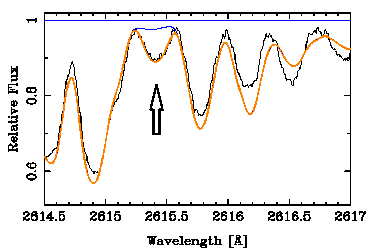
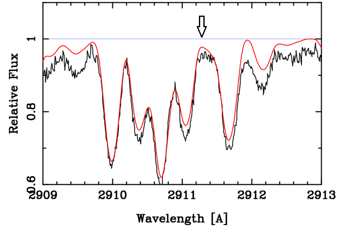
The wavelength of Lu II 2911.39A falls at an apparent high point in the continuum. No local minimum is observed, so we may use this region to set an upper limit to the lutetium abundance. However, for such a determination it is critical that the continuum be accurately set, as well as the oscillator strength be accurate. The region is shown in the plot below, using the continuum set for the entire region above 2000A, with no regard to this particular wavelength. The "high" in question is indicated by the arrow.
The Lu II 2615 line is the best defined of these features. We give it the highest weight, and adopt 1.6 dex for the lutetium excess.
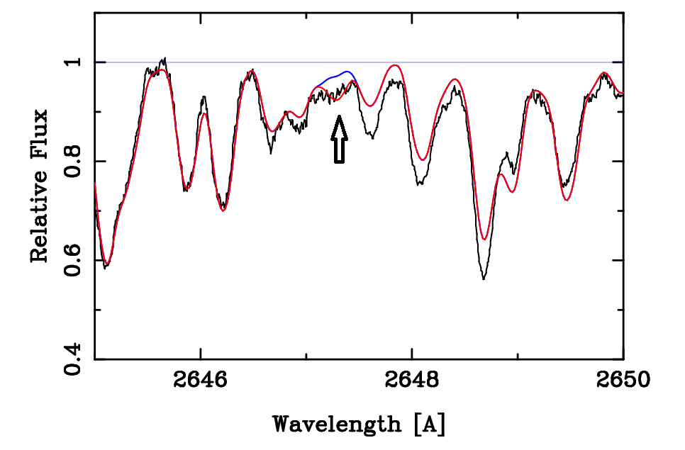
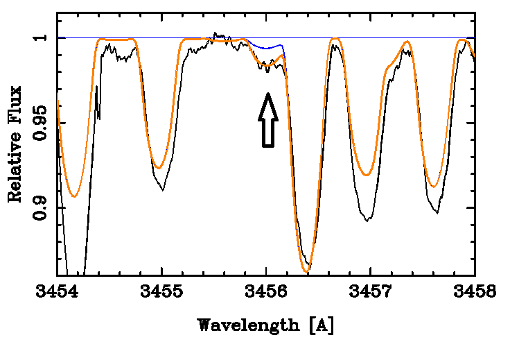
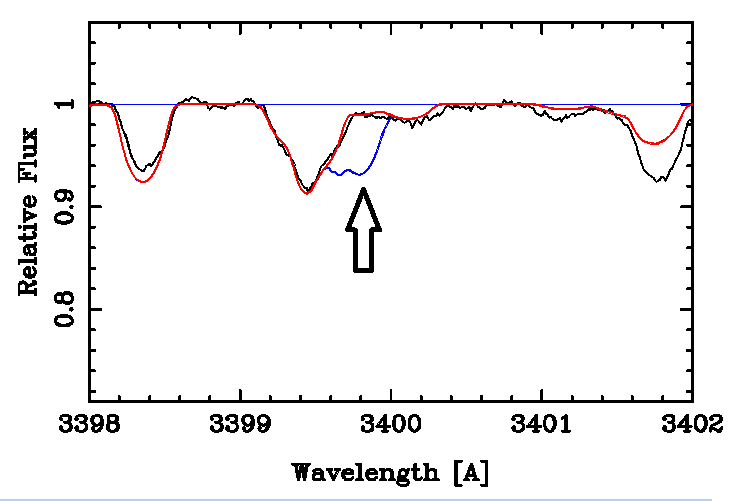
A comparable upper limit, 1.7 dex was derived from the complex at 3399.8A, which should contain the strong Hf II line at 3399.79A. The log(gf) is from Lawler et al. (2007, ApJS, 169, 120). Synthesis of this line is shown below.
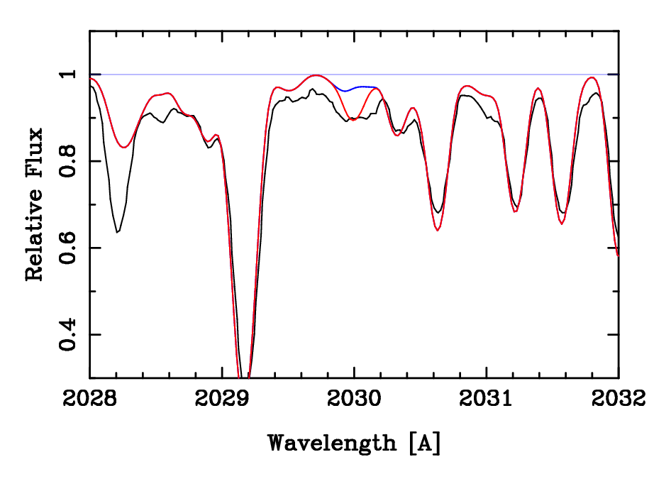
The strongest Hf II line in MCS is 2028.18. This line is apparently entered twice in VALD3 because the energy levels are different in MCS and modern sources. It is blended with Fe II 2028.197, for which the VALD3 oscillator strength (-4.208) is surely too small. The current Kurucz web page gives -2.755 for log(gf) for this line. Using the latter value, the stellar feature is slightly overfilled with a solar Hf abundance. This line is not useful for an abundance of hafnium!
The zero volt Hf II line at 3561.66A is also only useful for an upper limit. Synthesis with the solar value is shown in blue, but is hardly different from the orange, which was made with an abundance enhancement of +1.49 dex.
We have not sought Hf I or III. We adopt an 1.6 dex as an upper limit for hafnium.
Of the strong lines of Ta II, we examined two, at 2146.87 and 2400.63A. NIST does not not give oscillator strengths for these lines, but VALD3 gives Corliss-Bozman values. We suggest an uncertainties up to 1 dex for the two log(gf) values. More recent calculations are by Quinet, et al. A&A, 493, 711 (2009) but do not include these lines. We show calculations for the regions in question using solar Ta abundance (blue). The red line uses the CB oscillator strengths and abundance enhancements of 3.1 and 1.7 dex for the two lines, respectively.
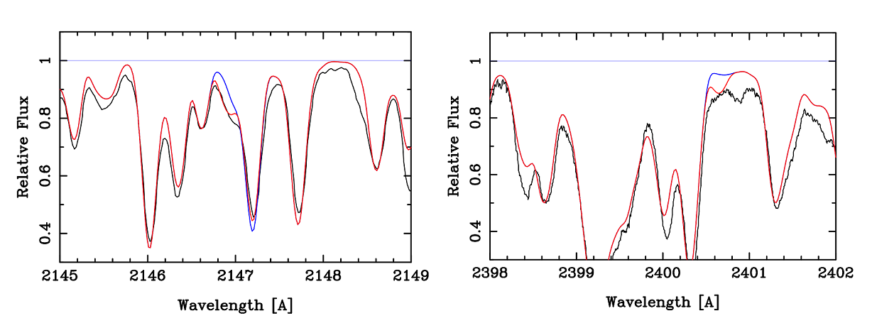
In both regions, there is the usual absorption that is unexplained, by our data base. The suggestion that some of this absorption could be due to Ta II is therefore tentative. We regard an excess of more than 3 dex as implausible, while the excess from the 2400-line, of 1.7 dex is in line with results from adjacent elements, plausible, and adopted here.
Our results differ from KS's in two respects. First, we use a more recent oscillator strength, from Nilsson, et al. (2008, Eur. Phys. J. D, 49, 13) The newer log(gf) is +0.18, much smaller than the one KS used, +2.63, from Kurucz and Peytremann (1975). Could this have been a typo? A second difference is that KS appears to get a reasonable profile fit with his Copernicus spectrum, while ours is obviously too narrow. Some of the difference may be in the observation. We find an upper limit of the tungston abundance of +1.8 dex. As the figure below shows, we must assume unknown lines fill in the missing absorption. We have no reason to believe the intrinsic profile of the W II line is unusually broad.
We get the same upper limit from the zero-volt line at 1951.05A.
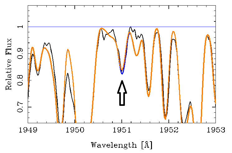
In this case, the blue line shows the effect of a tungston abundance enhancement of 1.5 dex over solar. The orange gives the calculation with solar tungston.
Our upper limit for tungston is 1.5 dex.
Rhenium remains one of the few unidentified elements in the sun (Grevesse, et al. 2015, A&A, 573, 27). The Jaschek's (1995) note several identifications in CP stars, of which, the identification in HR 465 is probably correct. A far more solid identification is in HD 65949 (Cowley et al. 2006, A&A, 455), where the hfs is clearly seen in several of the Re II lines. Wahlgren, et al. (1997, ApJ, 475, 380) sought Re II in the spectrum of Chi Lupi, concluding that the solar value was an appropriate upper limit. They gave detailed hyperfine structure of several lines from the Ultraviolet Multiplet 1 of Re II. The figure below is near the strongest of these lines, at 2275.25A. This figure was redrawn for a journal with colors that could be distinguished in a black/white print.
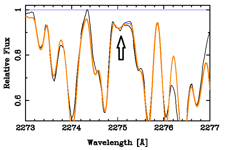
The brown line was made with a rhenium excess of 1.5 dex. The blue line, shows the calculation with solar rhenium. These calculations included the full hfs, as given by Wahlgren, et al (ApJ, 475,380, 1997).
We also looked at the strong Re II line at 2608.50, but could only conclude an upper limit for Re more than 2 dex above the solar value. An upper limit for rhenium of 1.5 dex is our estimate.
Among the stronger Os II lines, the line at 2194.39A appears to dominate a weak stellar feature measured at 2194.41A.
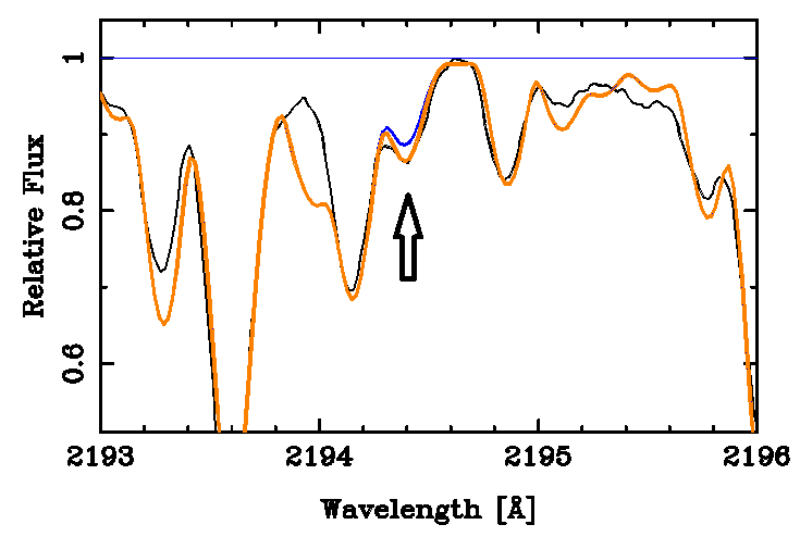
The blue line is made with solar osmium, and default values for other elements and oscillator strengths. The red line, which fits nicely is for an osmium excess of 1.5 dex.
The strongest Os II line in the NIST Handbook is 2067.21. The closest measured feature was at 2067.29A. It is mostly due to Si I at 2067.33. Unfortunately, both the oscillator strengths of many Si I lines are poorly known. Additionally, the silicon abundance in Sirius is at least 0.2 dex uncertain.
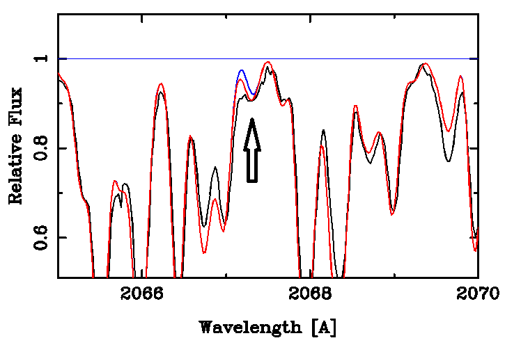
The blue line was made with a solar silicon abundance, and an oscillator strength for Si I 2067.33 of -1.80. The value from the Kurucz site was -1.56. The red line was calculated with a 1 dex enhancement for osmium. A larger f-value for Si I, or an increased silicon abundance could explain the absorption, leaving a small discrepancy (0.04A) with the wavelength measurement. That measurement is reasonably well explained by a blend.
The region nearest to the next strongest Os II line, at 2070.67A is overpredicted even if the osmium abundance is set to zero. We adjust the oscillator strength of the Fe II line in the region to get a rough fit to the observations with no osmium.
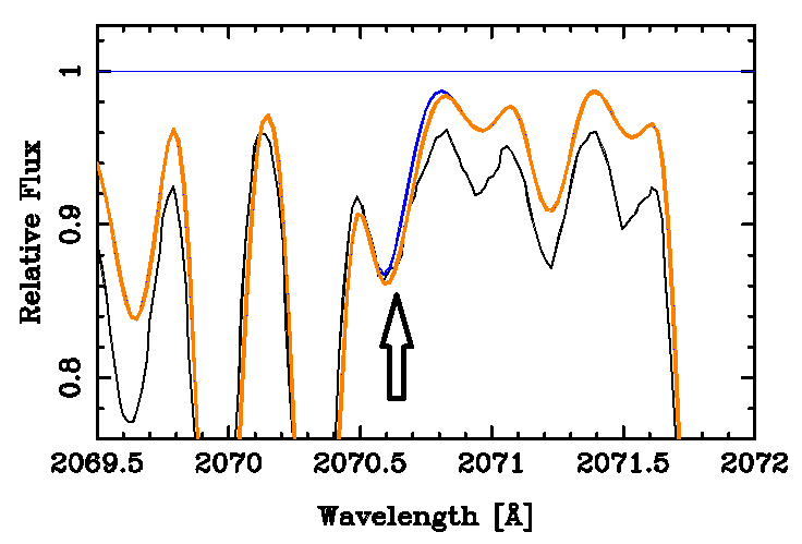
The calculation with no osmium is shown in blue. The orange line shows the effect of an osmium abundance of 1 dex above solar. Given the uncertainties, this excess is reasonable; an excess of 2 dex is not possible. The 2070.67 feature seems to indicate no osmium enhancement, contrary to our results for most of the neutron-addition elements of this study. This line is significantly stronger than that at 2194.39A which indicates a 1.5 dex enhancement of osmium. We therefore synthesized the region near the Os II line at 2282.26A. The feature shown by the red arrow is primarily Co II. We adjusted its oscillator strength downward for a slightly improved fit. Results are shown below.

The blue line shows the synthesis with solar osmium, and the orange an excess of +1 dex. We assume the oscillator strength of the 2070.67-line was too strong, or that oscillatory strengths of the Fe II and Ni II blends were too high. This would account for overfilling of the feature with no osmium. Oscillator strengths for Os are from Quinet, Palmeri, and Biemont (2006, A&A, 448, 1207). The VALD3 values for Os II should be updated.
We have three lines of Os II consistent with an excess of 1 dex for osmium. We adopt a 1 dex enhancement for osmium, and grade the determination 'f' for fair.
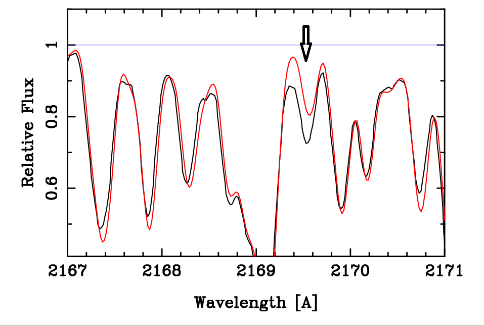
The strongest Ir II line, according to NIST is at 2169.42A, but is unclassified. Consequently, there is no gf-value for it, and its status as Ir II is uncertain. However, it is the only region where the observed profile is clearly underpredicted by the default abundances. The measured wavelength of the nearest stellar absorption feature is at 2169.63, so the stellar absorption cannot be Ir II alone.
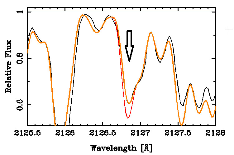
The figure below shows a synthesis of the region near the Ir II line at 2126.68A. It has a close blend to the red, which was overpredicted by our default strengths for Ni II 2126.84 and Fe II 2127.01. We chose to weaken the Fe II line to fit the red portion of the blend. The orange (or brown) plot was made with a solar abundance enhanced by 1 dex. It is marginally distinguishable from a plot with solar Ir. Therefore we show in red a plot with Ir enhanced by 2 dex, which we can clearly rule out. The oscillator strength for Ir II 2126.81 is Xu, Svandberg, Quinet, Palmeri, and Biemont (JQSRT, 104, 52, 2007), log(gf) = +0.11.
The stellar feature measured at 2144.366 was mentioned in connection with the cadmium identification and abundance. It cannot be fit without contributions from both elements, Cd II (2144.41) and Pt II (2144.25). The figure below shows an optimum fit (red), and one with solar-abundance platinum (blue). The optimum fit required a platinum excess of 1.41 dex. The moderate feature immediately to the violet of the Pt II blend was poorly fit with default abundances and transition probabilities. For purely cosmetic purposes, we made adjustments to the oscillator strengths of Cr III, 2144.15, Cr II 2144.08. Also, V II 2143.71 was calculated much too strong; the plot shows a calculation with its log(gf) reduced by 1 dex. log(gf) values
The figure below shows similar calculations of blended lines that contain substantial absorption by Pt II (1777.09, and 1883.06). Plots with solar platinum are again in blue. Excesses necessary for optimum fits were 2.0 dex for 1777.09 and 1.73 dex for 1883.03.
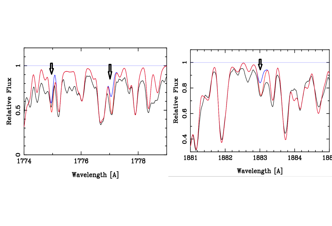
If we average the logarithms for the three platinum regions, the result is +1.7 dex. This is about a factor of three lower than found by YG.
Note that we used log(gf) = 0.103 rather than +1.27 as in VALD3, which we suspect is a typo (in the original source??)
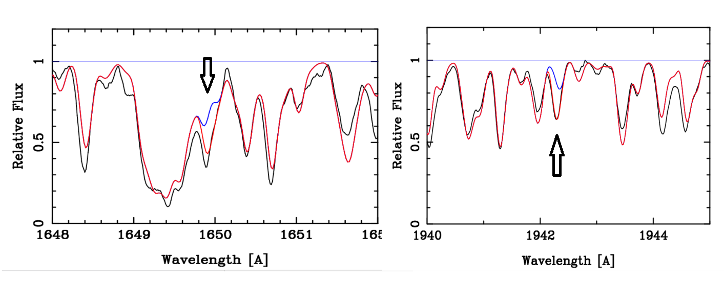
There is absorption in both regions that is not accounted for. In a few cases the predicted absorption is greater than the observed (black). However, for the positions of both the Hg II wavelengths, there is a significant amount of absorption that is missing unless a mercury abundance more than 1 dex above solar is assumed. In the case of the 1650-line, the needed excess is 1.9 dex, while for the 1942-line, it is 1.6 dex. We adopt 1.6 dex for the mercury excess.
Mercury identified by KS and YG and we confirm their result.
We know of no previous identification of thallium in Sirius. VALD3 does not contain any lines for Tl II. The adopted oscillator strength is from Curtis, L. J., Phys. Scr. 62, 31 (2000).
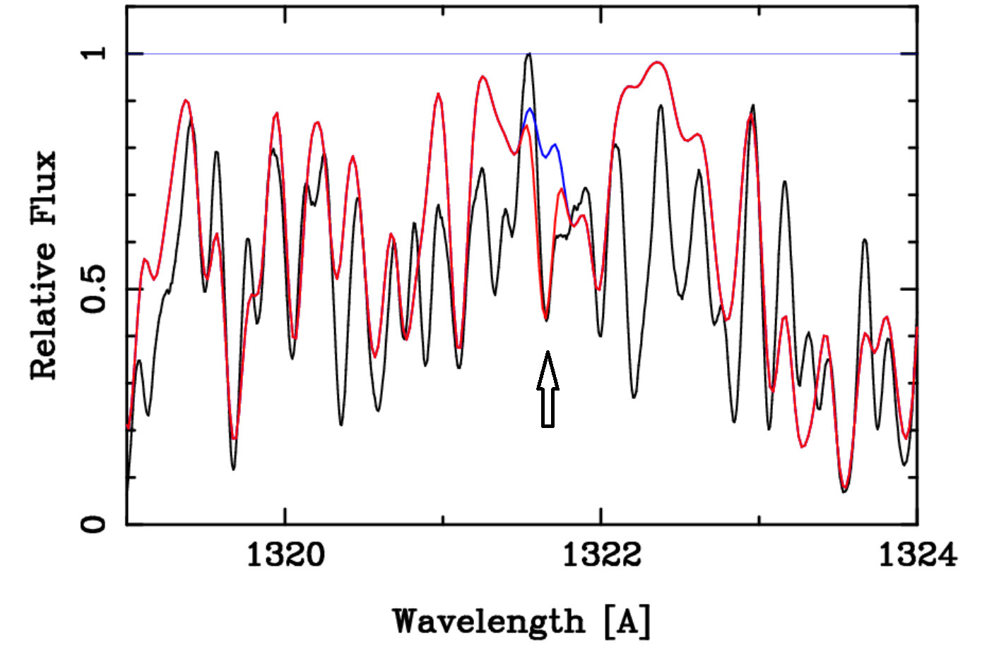
The region near 1322 is shown in the figure. Default parameters (microturbulence, instrumental resolution, adopted continuum, solar abundances) clearly do not begin to explain the observed absorption in this region. Moreover, the calculated line depths were much too small. In the figure, the calculation adopted Vturb = 4.4 rather than the Landstreet's 2.4 in order to approximate the depths of the observed lines.
A line was measured at 1321.68A, sufficiently far from the Tl II line (at 1321.64A) to be due to a blend, or the feature is not Tl II at all. The figure shows the result (red) of assuming an enhancement of thallium of 1.4 dex. The blue line shows the result of assuming a solar abundance.
The other zero-volt Tl II line is at 1908.62. A calculation omitting thallium altogether shows too much predicted absorption at this wavelength due to an Fe II line at 1908.68, with a VALD3 log(gf) of -0.790. This oscillator strength is a likely overestimate for this intersystem line (b4G_11/2 - 6F^o_9/2). If the log(gf) for the Fe II line is reduced by 1 dex, then a Tl excess of 1.4 dex is compatible with the observed spectrum.
A WCS run gives us the probability of finding an absorption within 0.04A of a wavelength near 1322A--it is 0.42. Thus the proximity of the stellar wavelength to the laboratory value cannot be used to strengthen the case for an identification. The strongest argument is plausibility. The apparent abundance for thallium, based on this single line (+1.4 dex) is withing the overall range for surrounding elements.
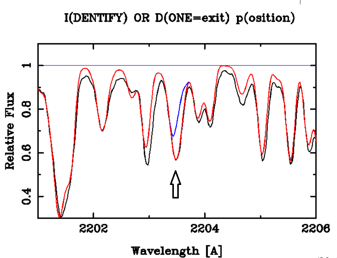
The 2203.53 feature was studied by KS. We confirm his finding that additional absorption is needed if one assumes a solar lead abundance, though we find a somewhat smaller excess is required. This is another one-line identification. The case for its validity is strengthened by the fact that the absorption feature is dominated by the assumed Pb II line. The fit shown here requires an excess of 1.6 dex above solar.
Oscillator strengths for bismuth are available from Palmeri, et al. (Phys. Scr. 63, 468, 2001), Wahlgren, et al. (ApJ, 551, 520, 2001), and Dolk, et al. (A&A, 388, 692,2002). Unfortunately we were unable to find a measurable feature that was plausibly dominated by Bi II. We synthesized regions near lines at 1436.81, 1791.84, and 1902.34A. In all cases, we found only upper limits to the bismuth abundance. The figure shows one example.
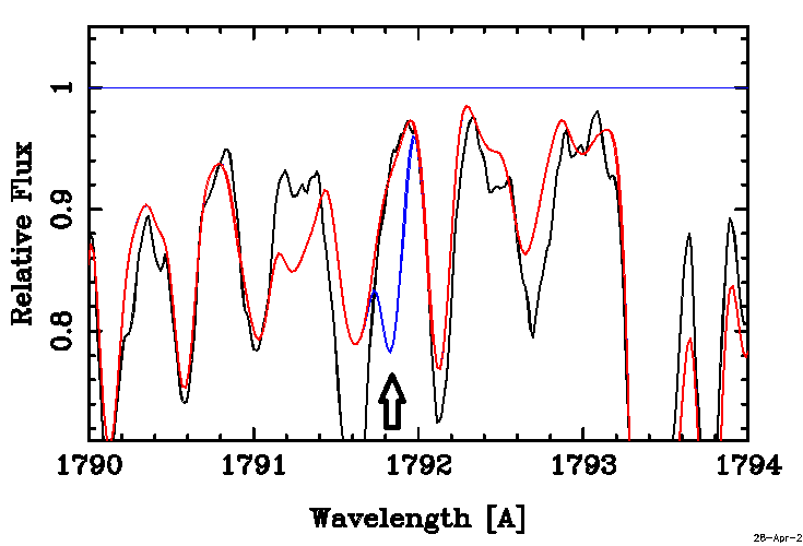
Upper limits for 1436 and 1902 were respectively 1.1 and 2.0 dex. Granted the overall uncertainty] of the calculation, an average of these upper limits is reasonable. We adopt 1.6 dex, which is also the value from the 1791 line.
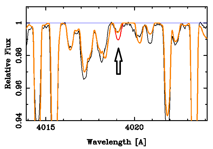
In the figure above, the orange line gives the synthesis with thorium 1.6 dex above solar, while the red is for thorium up by 2.6 dex. Transition probabilities are available for Th III from the work of Biemont, et al. 2002, Ap. J., 567, 1276. The strongest lines are unfortunately in the deep ultraviolet (1307.44 - 1463.35A); using 1307.44 and 1356.92, we could only exclude thorium excesses above about 3 dex. For thorium, we adopt an upper limit of +1.6 dex.
There are no U III lines on the NIST site. Blaise and Wyart give a number of U III wavelengths with intensities (Energy Levels and Atomic Spectra of Actinides, in International Tables of Selected Constants, Vol. 20, Centre Nationale de la Recherche Scientifique, Paris, 1992). The strongest U III line is at 3565.73A. We found no oscillator strengths for U III. We therefore worked with log(gf) = 0.3 for this strongest of the Blaise-Wyart lines. Synthesis is shown below.
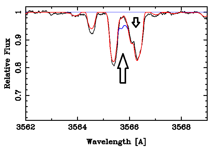
Adjustments were made to Fe II and Ni II lines in the region shown by the wide, downware-pointing arrow in order to fit the blend. The value of log(gf) for Fe II 3566.06 was changed from -2.59 to -2.00, while that for Ni II 3566.17 was changed from -0.24 to +0.24.) This was deemed advisable as the blend could contribute at the position of the putative U III absorption. In making these adjustments, we assumed no uranium contribution.
The red spectrum was calculated with an enhancement of uranium of +3.0 dex. The difference from assuming no uranium is marginally detectable (ca. 0.5%). The blue line shows a calculation with uranium enhanced by 4 dex. The adopted upper limit will scale with the log(gf) of the U III line. We currently adopt an upper limit of 3 dex.
YG obtained abundance excesses for Pb, Bi, Th, and U of 3 or more dex. We cannot comfirm these excesses.