Learning Resources

Solved Problem - Example CD13-1: RTD Calculations for a Series Reaction

Consider the reaction  
   

image 13eq53.gif


occurring in two different reactors with the same mean residence time tm=1.26 min, but with the following residence-time distributions which are quite different:

(a) Calculate the conversion predicted by an ideal
  1. PFR.
  2. CSTR.
(b) Fit a polynomial to each RTD (Figures CDE13-1.1 and CDE13-1.2). Note: These curves are identical to Figures E13-9.1 and E13-9.2 in the text.


Figure CDE13-1.1
E1 (t ):asymmetric distribution.


Figure CDE13-1.2
E
2 (t ): bimodal distribution.


(c) For the multiple reaction sequence given above, determine the product distribution in each reactor for 1. The segregation model. 2. The maximum mixedness model.


Solution

PFR
Combining the mole balance and rate laws for a PFR reactor, we have


image 13eq54.gif


(CDE13-1.1)


(CDE13-1.2)


(CDE13-1.3)

The initial conditions are V = 0, CA = 1, CB = CC = 0. In order to compare the performance of the different models and different RTDs, the mean residence time,greekt, was set equal to 1.26 min.

The POLYMATH program used to solve this PFR system is shown in Table CDE13-1.1. The solution is CA = 0.284, CB = 0.357, CC = 0.359, X = 71.6%.


Table CDE13-1.1.
Polymath Program for Reactions in a Series in a PFR


CSTR
The mole balances on A, B, and C for a CSTR are


image 13eq55.gif


(CDE13-1.4)


(CDE13-1.5)


(CDE13-1.6)
   

The equations can be solved with a nonlinear equation solver. Again,greektwas set to 1.26 min for comparison reasons.


The POLYMATH program for the CSTR model is shown in Table CDE13-1.2.The solution is CA = 0.443, CB = 0.247, CC = 0.311, X = 55.7%


Table CDE13-1.2.
Polymath Program for Reactions in a Series In a CSTR


Segregation Model
Combining the mole balance and rate laws for a constant-volume batch reactor, we have:

For the globules


image 13eq56.gif


(CDE13-1.7)


(CDE13-1.8)


(CDE13-1.9)
For the exit concentrations  
   

image 13eq57.gif


(CDE13-1.10)


(CDE13-1.11)


(CDE13-1.12)
   

The initial conditions are t = 0, CA = 1, CB = CC = 0 The POLYMATH program used to solve these equations is shown in Table CDE13-1.3 forE1(t) (1) and in Table CDE13-1.4 for E2(t) (2).The results are listed in Table CDE13-1.5.


Table CDE13-1.3.
POLYMATH Program for Segregation Model with Asymmetric RTD


Table CDE13-1.4.
POLYMATH Program for Segregation Model with Bimodal Distribution


image 13eq58.gif


Maximum Mixedness Model
The equations describing the variations in concentrations with position (life expectancy) are


image 13eq59.gif


(CDE13-1.13)


(CDE13-1.14)


(CDE13-1.15)

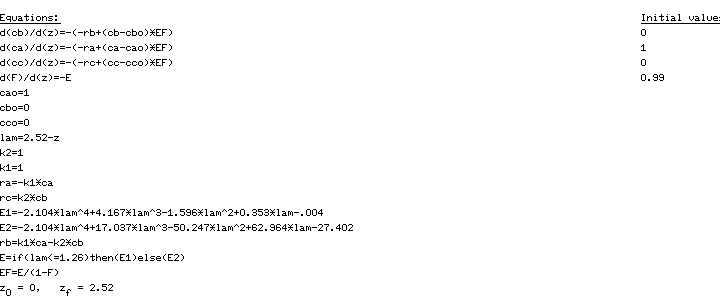
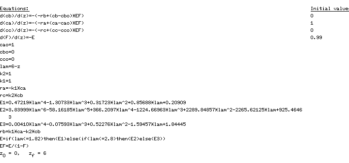
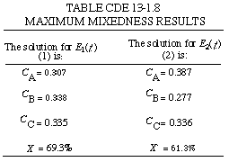
The POLYMATH program is shown in Table CDE13-1.6 for E1(t) (1)and in Table CDE13-1.7 for (2). The results are listed in Table CDE13-1.8.


Table CDE13-1.6.
POLYMATH Program for Maximum Mixedness Model with Asymmetric RTD


Table CDE13-1.7.
POLYMATH Program for Maximum Mixedness Model with Bimodal Distribution


image 13eq60.gif


Summary: Example CD13-1


image 13eq61.gif


Additional Tables for Example 13-9

Table CDE13-9.5.
POLYMATH Program for Segregation Model with Bimodal Distribution (Multiple Reactions)


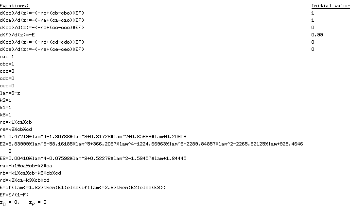
Table CDE13-9.6
POLYMATH Program for Maximum Mixedness Model with Asymmetric RTD (Multiple Reactions)