Chapter 14 - Professional Reference Shelf

Professional Reference Shelf

R14.1 Derivation of Equation for Taylor-Aris Dispersion

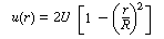
	In a laminar flow reactor we know that the axial velocity varies in the radial direction according to the Hagen-Poiseuille equation:



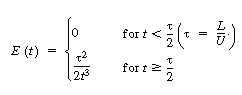
	where U is the average velocity. For laminar flow we saw that the RTD function E(t) was given by



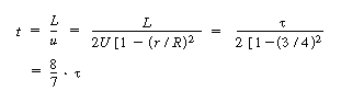
	In arriving at this distribution E(t) it was assumed that there was no transfer of molecules in the radial direction between streamlines. Consequently, with the aid of Equation (13-43), we know that the molecules on the center streamline (r = 0) exited the reactor at a time t = / 2, and molecules traveling on the streamline at r = 3R/4 exited the reactor at time

		(13-43)

	The question now arises: What would happen if some of the molecules traveling on the streamline at r = 3R/4 jumped (i.e., diffused) to the streamline at r = 0? The answer is that they would exit sooner than if they had stayed on the streamline at r = 3R/4. Analogously, if some of the molecules from the faster streamline at r = 0 jumped (i.e., diffused) to the streamline at r = 3R/4, they would take a longer time to exit (Figure R14.1-1). In addition to the molecules diffusing between streamlines, they can also move forward or backward relative to the average fluid velocity by molecular diffusion (Fick's law). With both axial and radial diffusion occurring, the question arises as to what will be the distribution of residence times when molecules are transported between and along streamlines by diffusion. To answer this question we will derive an equation for the axial dispersion coefficient, D _a , that accounts for the axial and radial diffusion mechanisms. In deriving D _a , which is referred to as the Aris-Taylor dispersion coefficient, we closely follow the development given by Brenner and Edwards. ¹

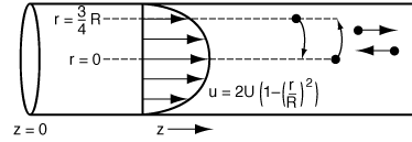
	Figure R14.1-1 Radial diffusion in laminar flow

	The convective-diffusion equation for solute (e.g., tracer) transport in both the axial and radial direction is

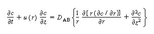
		(R14.1-1)
	We are going to change the variable in the axial direction z to, which corresponds to an observer moving with the fluid

		(R14.1-2)

	A value of = 0 corresponds to an observer moving with the fluid on the center streamline. Using the chain rule, we obtain

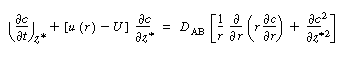
		(R14.1-3)

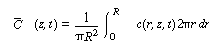
	Because we want to know the concentrations and conversions at the exit to the reactor, we are really only interested in the average axial concentration , which is given by

		(R14.1-4)

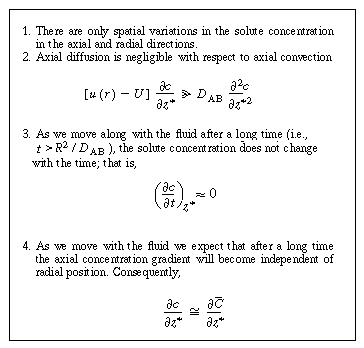
	Consequently, we are going to solve Equation (R14.1-3) for the solution concentration as a function of r and then substitute the solution c(r, z, t) into Equation (R14.1-4) to find (z, t). To solve equations (R14.1-1) to (R14.1-4) to determine the Aris-Taylor dispersion coefficient, we make the following four assumptions:



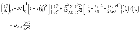
	We now apply the preceding approximations to Equation (R14.1-4) to arrive at the following equation:

		(R14.1-5)

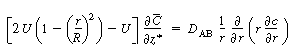
	Because is independent of r, Equation (R14.1-5) can be rearranged and integrated with respect to r:



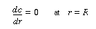
	Symmetry conditions dictate that at r = 0,, and therefore the constant of integration, K ₁ , is zero. After dividing both sides by r, a second integration yields

		(R14.1-6)
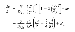
	The constant of integration K ₂ is independent of r and can be evaluated using the equation for the average concentration:


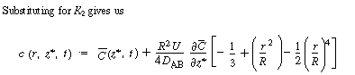		(R14.1-7)
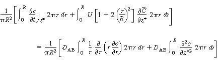
	The final step to arrive at the celebrated Aris-Taylor dispersion coefficient,D,* is to multiply Equation (R14.1-3) by the differential cross-sectional area 2r dr and carry out the integration over the tubular reactor radius R:



	By changing the order of differentiation and integration for the first and last terms and recalling Equation (R14.1-4) gives

		(R14.1-8)

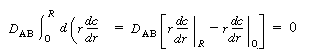
	Because there is no transport of solute through the tube wall,



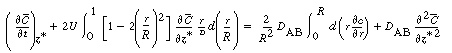
	Integrating the first term on the right-hand side of Equation (R14.1-8) along with the preceding boundary condition above gives

		(R14.1-9)
	Next we differentiate Equation (R14.1-7) with respect to and substitute it into the second term on the left-hand side of Equation (R14.1-8) to yield

		(R14.1-10)

	Carrying out the integration between 0 and 1 (r = R) gives

		(R14.1-10)

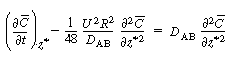
	Changing our variable back to z gives

		(R14.1-11)

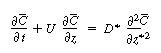
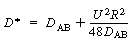
	where D* is the Aris-Taylor dispersion coefficient:

Aris-Taylor dispersion coefficient		(R14.1-12)

	_{That is, for laminar flow in a pipe}



	Figure 14.5 shows the dispersion coefficient D* in terms of the ratio 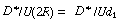as a function of the product of the Reynolds and Schmidt numbers.