In this section we will step you through the HCN isomerization example and along the way we will explain all the available options and what they all mean superficially and in-depth.

For a printable version of this text click here Cerius² instructions (.doc, .pdf)

1. In the main Cerius2 window:

change form stick view to ball and stick view by left clicking on the light brown box labeled stick directly below the drop down menu bar.

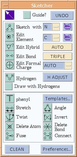
2. In the drop down menu left click on build select 3D-sketcher and the sketcher window will open and look like this:

3. In the sketcher window left click on the sketch button that looks like this: .

4. Be sure that directly to the right of the sketch button the carbon atom is selected, indicating that you will be drawing a carbon atom.

5. Draw a carbon atom by left clicking in the Cerius2 Models window once and then moving the pointer outside the model window. If you happen to make a mistake left click on the delete atom button and left click in the model window on the atom that you wish to delete.
6. Next to the sketch button in the sketch window left click on the drop down button next to the blue box where there should presently be a C and change to a N indicating that you will be drawing a nitrogen atom next.

7. Left click in the model window and then remove the pointer once again.

8. Draw a hydrogen atom in the model window using the same technique.
9. To bond these atoms select the edit bond button in the sketch window and to the right of the edit bond button left click and hold on the light brown button labeled single. A drop down menu should appear containing all available bond types. Select single bond and move to the model window and left click on the H then on the C. You should have drawn a single bond between them.

10. Now change to a triple bond and draw the bond between the carbon and the nitrogen.

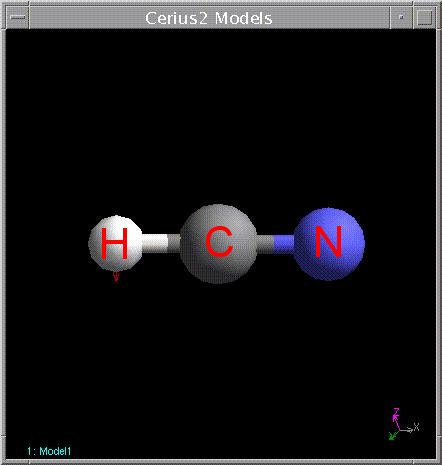
11. Left click and hold on the clean button in the lower left of the sketch window until the HCN molecule stops moving, indicating that the program has roughly minimized the molecules energy. Your HCN molecule should look something like this:

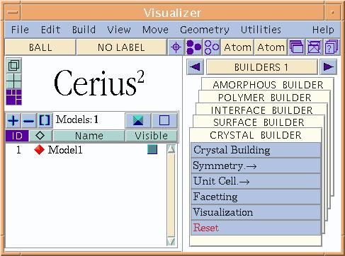
Possibly with a slightly longer CN bond since the clean button does not do a very good job of minimizing the energy of the molecule.12. In the right portion of the visualizer window left click and hold on the light brown bar that is labeled BUILDERS1 and select from the menu that appears QUANTUM1.

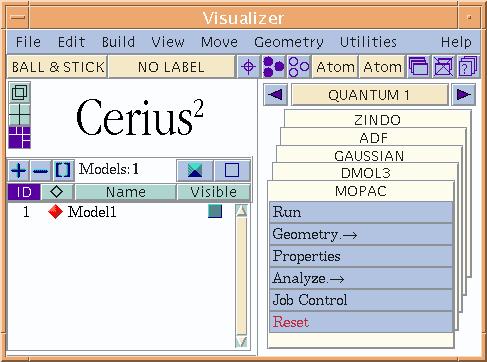
13. In the tiled windows below left click on the MOPAC tab, sending it to the front. The visualizer window should now look like this:

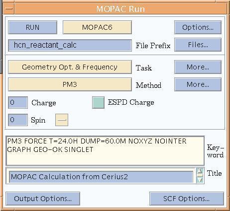
14. Now left click on Run in the blue MOPAC menus, another window labeled MOPAC Run window will pop up. This is where you will be able to tailor the calculations that you will be doing on these molecules. The window will look like this, here the file name was changed, the calculation function was changed to geometry optimization and frequency, and the calculation method was changed to PM3. You will learn how to do that in the next steps.

15. First we will change the file name that this run will be saved under by left clicking in the blue box below the run button in the upper left hand corner, presently the name of the file should be mopac.

16. Change the file name to a suitable file name for the reactant calculations (i.e., hcn_reactant, do not use spaces in the file name) and hit enter.

17. Let us explore a bit before we start calculating:

1. Left click on the options button in the upper left of the MOPAC Run window

2. The MOPAC Run Options window will pop up.

3. Here you can set a time limit for the calculation that the computer will run, the default is 24 hours which if these calculations take that long something has gone wrong, so go ahead and leave these settings as they are.

4. Also some technical issues such as using a restart file to setup calculations where you left off, a selection that enables you to stop and restart the program if need be, also an option to check the input to check for errors in the setup before the program is run, and other self-explanatory options.

5. Go ahead and close this window. You may do this by double clicking on the small box in the upper left hand corner of the window you want to close.

6. Left click on the More... button below the files button

7. Here we can select what kind of calculation task we wish to perform and its associated options.

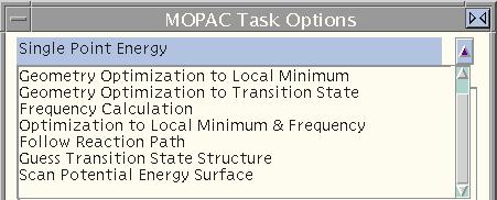
8. At the top of the task options window you will find a blue drop down window that contains all of the calculations that you can perform. Left click on the arrow to the right of the drop down menu. Here we see we have plenty of calculation functions to choose from:

lets quickly explain all of the functions:

1. single point energy : This function calculates molecular orbitals, heat of formation, and requested thermodynamic quantities for the molecule drawn in the modeling window. This calculation does not optimize the geometry of the molecule.
2. geometry optimization to a local minimum : This function finds a local minimum in the molecules energy. The program systematically changes the spatial configuration of the molecule, calculates the overall energy change of the new spatial configuration, and eventually finds the lowest energy configuration of the molecule.
3. geometry optimization to transition state : This function finds a probable transition state by changing the spatial geometry of the molecule in such a way as to increase the total energy of the molecule. Coupled with a search for an imaginary frequency in the direction of the reaction the program can identify a probable transition state.
4. frequency calculation : This function calculates the vibrations, rotations, and translation frequencies for the molecule.
5. optimization to a local minimum and frequency : This function is just a combination of the geometry optimization to a local minimum and the frequency calculation.
6. follow reaction path : This function calculates the energy of the molecule from the local minimum through the transition state and on to the products local minimum. This function requires a geometry optimization to a transition state be run first to find the transition state.
7. guess transition state structure : This function uses a data base of reactions to make an educated guess as to what the transition state of a reaction may be.
8. scan potential energy surface : This function varies two spatial parameters that are set by the user and creates a three dimensional potential energy surface that relates for example two bond distances and their respective total molecular energy.

9. Go ahead and select the geometry optimization to a local minimum and frequency calculation, and click on the blue box next to thermochemistry calculation to have the program calculate the thermodynamic quantities associated with the molecule. Then close the window.

18. Left click and hold on the light brown button below the calculation function chooser, here we can select different types of semi-empirical calculation methods such as PM3, AM1, MNDO, and MINDO3:

Quick background on semi-empirical calculation methods: Semi-empirical methods are simplified forms of the Hartree-Fock calculation methods. These calculations utilize empirical data combined with fitting parameters to account for the simplifications made. In the original Hartree-Fock calculations the energy associated with atomic orbital overlap (two electron integrals) were very time consuming to calculate. Back when computers were still slow these two electron integrals were removed and replaced with empirical data modified by a set of fitting constants. These terms (empirical data multiplied by fitting constants) approximated the energy contained in the atomic orbital overlap for each atom, thus making the semi-empirical calculations very time efficient and fairly accurate.

MNDO : Modified Neglect of Differential Overlap - A semi-empirical hamiltonian for multi-center repulsion integrals. This is based off of the neglect of differential diatomic overlap.

MINDO : Modified Intermediate Neglect of Differential Overlap - A semi-empirical hamiltonian that does not use analytic solutions, but empirical data as the set of parameters for the repulsion integral. This method allows for the atomic orbital differences.

PM3 : Utilizes NDDO (Neglect of Differential Diatomic Overlap) with up to 18 independent empirical fitting parameters for each element. Incorporates more terms related to electron interaction. Generally one of the most accurate methods.

AM1 : Utilizes NDDO with 10-19 empirical fitting parameters. Incorporates more terms related to electron interaction. Generally one of the most accurate methods.

Select the PM3 calculation method.

19. Further down in the MOPAC Run window you will find the electron spin, this specifies how many unpaired electrons are present in the molecule. For our HCN molecule there are no unpaired electrons so leave the spin as zero.

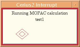
20. After all of the options you want are selected left click on the blue RUN button in the upper left had corner of the Run window. A small pop up window should appear as the computer calculates [show window]

21. When the run window disappears the calculation is done. A graph window will pop up that contains the infrared spectra of the molecule. In the visualizer window in the right hand portion left click and hold on the analyze button. The properties that you may analyze are displayed here.

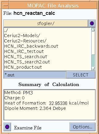
22. Chose files, another pop-up window will appear:

with the heat of formation and dipole moment shown in the lower portion. Left click on the Examine File button to show a text form of the output of the calculation. Scroll through the data and record the heat of formation, the enthalpy, the heat capacity, and the entropy all at 300K. We will be using this later.

23. Left click and hold on the analyze button and select the vibrations.

24. With the model window visible select a frequency and left click the green animate button below the frequencies to animate the vibrations. To stop the vibration animation just left click on another frequency. These are the bends, stretches, and rotations that the molecule would be doing in its natural state.

25. Go ahead and close the vibrations window.

26. Now there are some very interesting molecular orbitals that we can view, but first for clarity we are going to change a viewing parameter so we can see the atoms a bit more clearly within the molecular orbitals. Left click on surfaces under the analyze section of the blue MOPAC menus, there is a transparency % selection in the lower left corner or the surfaces window. Type 50 in the blue box and hit enter, then close the window. Then left click and hold on analyze again and select orbitals. Another pop up window should appear showing the different orbitals and their corresponding energies.

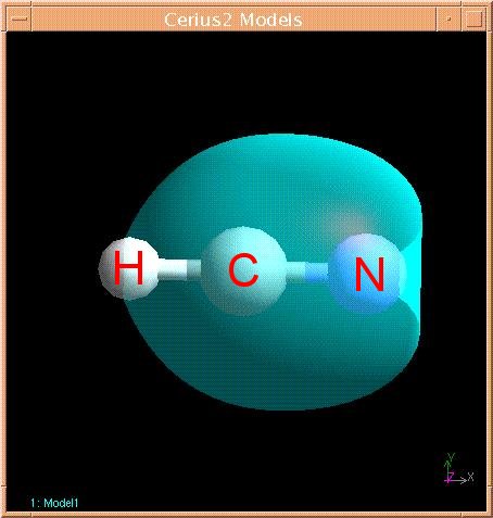
27. Left click on the first orbital and then left click on the calculate button in the upper left hand corner of the orbitals window. Another window will pop up and show that the orbital is being calculated. After the calculation is finished the HCN molecule in the models window should be surrounded by a somewhat spherical light blue orbital. The first orbital should look like this:

28. Left click on each orbital and calculate each to see what they look like, there are some really cool looking ones, then go ahead and close the orbitals window.

29. Now lets go ahead and move on to the transition state calculations.

Now on to the transition state calculations.