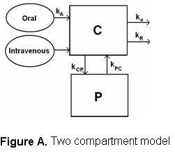
Many drug delivery studies use simplified lumping by considering only two compartments for intravenous injection of the drug and three compartments to include the stomach when the drug is taken orally. The two compartment model has a central compartment, C, consisting of blood and highly perfused organs such as the liver, kidney, lungs, etc., and also a peripheral compartment, P, consisting of the less perfused organs such as muscle and tissue.
Here kCP and kPC are the first order inter-compartmental distribution constants, kA is the rate constant for absorption from the stomach into the central compartment, kR is the drug's specific metabolism rate constant and ke is the elimination rate constant, all with units of reciprocal hours. Oral administration is sometimes considered a three compartment model because of time it takes the drug to dissolve and enter the blood stream, i.e., central compartment.
We now consider the case where drug dose m0 usually in milligrams (mg), is injected intravenously into the central compartment. We are going to let
k0 = kR + ke + kCP
since all are first order processes. The mass balances on the drug are in the central and peripheral compartments are
Central: ![]() , when t = 0 then mC = m0
(1)
, when t = 0 then mC = m0
(1)
Peripheral: ![]() , when t = 0 then mP =
0
(2)
, when t = 0 then mP =
0
(2)
where mc and mp are the mass of drug (e.g., milligram) in the central and peripheral compartments, respectively. These equations are easily solved by recognizing that the one of the form to
(1) ![]()
![]()
![]() (3)
(3)
(2) ![]()
![]()
![]() (4)
(4)
Or in Matrix Notation

![]()
![]() and
and ![]() (5)
(5)
where
 (6)
(6)
![]() (7)
(7)
![]() (8)
(8)
For our system
![]() (9)
(9)
![]() (10)
(10)
![]() (11)
(11)
t = 0 x = x0 and y =
y0 we get ![]() and
and ![]()
 (12),(13)
If y0 = 0
 (14)
(14)
![]() (15)
(15)
Evaluating the constants ![]() ,
, ![]() , and c for
our system.
, and c for
our system.
where
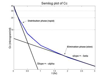
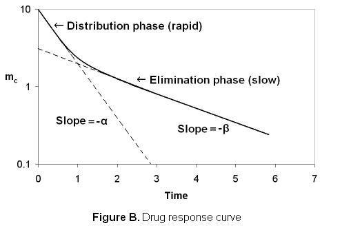
A typical biexponential response curve is shown in Figure B for the drug in the central compartment.
Here one observes a rapid
decay (![]() ) of drug concentration from the central compartment as it is being distributed to
the other compartments. This phase is
) of drug concentration from the central compartment as it is being distributed to
the other compartments. This phase is ![]() followed by a slow decay (
followed by a slow decay (![]() ) elimination phase. The actual distribution curves can be seen for ampicilin, diazepam and other
drugs by plotting the data in Problem P7-26B. Here the drug concentrations are just the mass divided by
the compartment volume, i.e.,
) elimination phase. The actual distribution curves can be seen for ampicilin, diazepam and other
drugs by plotting the data in Problem P7-26B. Here the drug concentrations are just the mass divided by
the compartment volume, i.e., ![]() and
and
![]() .
.
![]() Intravenous
Injection of 2-pyridinivens adoximine methochloride (2-PAM)
Intravenous
Injection of 2-pyridinivens adoximine methochloride (2-PAM)
The drug 2-PAM is given as an antidote for the ingestion of herbicides and pesticides such as parathion. An aqueous solution 2-PAM is injected intravenously. We will use the two compartment model discussed above where 2-PAM is injected into the central compartment. Assume that the volume of body fluid accessible to exchange per kg of the body weight is 250 ml. The concentration of 2-PAM is shown as a function of time in the table below.
2-pyridinium adoximine methochloride 10 mg/kg intravenous dose
|
0.1 |
0.2 |
0.3 |
0.5 |
0.7 |
1 |
1.5 |
2.0 |
3.0 |
||
|
C(mg/ml) |
30 |
25 |
18 |
14 |
8 |
6 |
4 |
2.8 |
2 |
1.2 |
Determine the distribution and elimination parameters and then use POLYMATH to solve for the concentrations of 2-PAM in both the central and the peripheral compartments as a function of time. Vary different parameters and compare analytically and numerically.
Solution:
First we will plot the concentration of 2-PAM as a function of time
|
|
|
|
Figure E1: CC vs t |
Figure E1: CC vs t in semilog scale |
Next we calculate the initial concentration of 2-PAM in the central compartment.
Since we have 10 mg of drug per kg of the human body, and for each kg we have 250 ml of fluid volume accessible for exchange,
Initial concentration of the drug = ![]()
So, we start with Co = 40 microgram/ml at t = 0. Expressing equations (16) and (17) in terms of concentrations of the drug in central and peripheral compartments, we have
|
|
|
|
We now use the polymath non-linear regression program to find ![]() ,
,
![]() and k0 from the given data series of CC
and k0 from the given data series of CC
POLYMATH 5.0 Results
Nonlinear regression (L-M)
Model: Cc = 40 * ( (k0-b)*exp(-a*t) + (a-k0)*exp(-b*t) )/(a-b)
Variable Ini guess Calc Value
k0 2. 5.0223943
b 4. 7.0006187
a 0.5 1.0869165
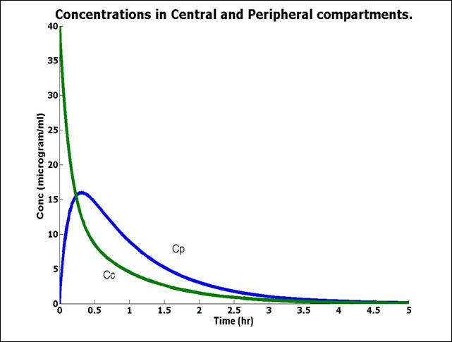
Now that we have the constants, we now plot the concentration of 2-PAM in the central compartment, and the peripheral compartment as a function of time using the Polymath.
Polymath Code:
ODE Report (RKF45)
Differential equations as entered by the user
[1] d(Cc)/d(t) = -k0*Cc+kpc*Cp
[2] d(Cp)/d(t) = kcp*Cc-kpc*Cp
Explicit equations as entered by the user
[1] ke = 2.511
[2] kpc = 3.0651
[3] kcp = 3.936
[4] kr = 2.511
[5] k0 = kr+ke
(Change the values of the four rate constants and genenerate plots.)
Click here to access the Polymath Program.
Model Parameters:
k0 = 5.022
kpc = ![]() = 3.065
= 3.065
kCP = ![]() = 3.936
= 3.936
(ke + kr) = ![]() =1.087
=1.087
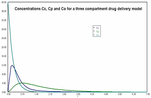
Three Compartment Model :
This model is used for oral drug administration. Here we assume the drug is taken all at once orally and goes directly to the stomach. The rate of adsorption from the stomach onto the central compartment ir rArs kaC0 where kA is the adsorption constant and C0 is the concentration in the stomach. We also need to add a balance on the drug concentration in the stomach:
![]()
The initial concentration of the drug in the stomach is taken to be 40 micrograms per mL.
For the three compartment model, we have the differential equations for the Central, Peripheral and the Oral compartment as :
![]() (20)
(20)
![]() (21)
(21)
![]() (22)
(22)
These can be solved using POLYMATH to produce the concentration plots once the required rate constants are plugged in.
ODE Report (RKF45)
Differential equations as entered by the user
[1] d(Cc)/d(t) = -(ke+kr+kcp)*Cc + kpc*Cp + ka*Co
[2] d(Cp)/d(t) = -kpc*Cp + kcp*Cc
[3] d(Co)/d(t) = -ka * Co
Explicit equations as entered by the user
[1] ke = 2.0
[2] kr = 3.0
[3] kcp = 1.0
[4] kpc = 1.0
[5] ka = 4.0
Comments
[1] d(Cc)/d(t) = -(ke+kr+kcp)*Cc + kpc*Cp + ka*Co
Concentration of drug in Central Compartment
[2] d(Cp)/d(t) = -kpc*Cp + kcp*Cc
Concentration of drug in Peripheral Compartment
[3] d(Co)/d(t) = -ka * Co
Concentration of drug in Oral Compartment
Click here to access the Polymath Program.