Tert-Amyl Methyl Ether (TAME) is an oxygenated additive for green gasolines. Besides its use as an octane enhancer, it also improves the combustion of gasoline and reduces the CO and HC (and, in a smaller extent, the NOx) automobile exhaust emissions. Due to the environmental concerns related to those emissions, this and other ethers (MTBE, ETBE, TAEE) have been lately studied intensively.
TAME is currently catalytically produced in the liquid phase by the reaction of methanol (MeOH) and the isoamylenes 2-methyl-1-butene (2M1B) and 2-methyl-2-butene (2M2B). There are three simultaneous equilibrium reactions in the formation and splitting of TAME: the two etherification reactions and the isomerization between the isoamylenes:
![]() (1)
(1)
![]() (2)
(2)
![]() (3)
(3)
These reactions are to be carried out in a plug flow reactor and a membrane reactor in which MeOH is fed uniformly through the sides.
For isothermal operation:
a) Plot the concentration profiles for a 10 m3 PFR.
b) Vary the entering temperature, T0, and plot the exit concentrations as a function of T0.
For a reactor with heat exchange (U = 10 J.m-2.s-1.K-1):
c) Plot the temperature and concentration profiles for an entering temperature of 353 K
d) Repeat (a) through (c) for a membrane reactor.
Additional information for solving the problem
· Thermodynamic equilibrium constants, activity based (Vilarinho Ferreira and Loureiro, 2001)
 (I.1)
(I.1)
 (I.2)
(I.2)
![]() (I.3)
(I.3)
with: T in Kelvin
· Kinetic constants for the direct reactions (Kiviranta-Pääkkönen et al., 1998)
 (I.4)
(I.4)
 (I.5)
(I.5)
 (I.6)
(I.6)
with: k in mol.![]() .s-1
.s-1
T in Kelvin
R = 8.314 J.mol-1.K-1
· Adsorption constants for each component, activity based (calculated and adapted from Oktar et al., 1999)
 , 1B = 2M1B (I.7)
 , 2B = 2M2B (I.8)
 , M = MeOH (I.9)
 , T = TAME (I.10)
with: T in Kelvin
· Heat of reaction (Vilarinho Ferreira and Loureiro, 2001)
![]() = - 41.708 kJ.mol-1
= - 41.708 kJ.mol-1
![]() = - 30.981 kJ.mol-1
= - 30.981 kJ.mol-1
![]() = - 10.727 kJ.mol-1
= - 10.727 kJ.mol-1
· Bulk density and bed porosity
The PFR is filled with a macroreticular strong cation ion-exchange resin in hydrogen form (Amberlyst 15 Wet, Rohm & Haas).
The bulk density is: ![]()
The bed porosity is: e = 0.4
· Rate equations for the formation of each component (Vilarinho Ferreira and Loureiro, 2001)
 (I.11)
 (I.12)
![]() (I.13)
(I.13)
![]() (I.14)
(I.14)
with: r in mol.![]() .s-1
.s-1
ai stands for the activity of component i in the liquid phase, calculated by the following equation:
![]() (I.15)
(I.15)
where gi is the activity coefficient of component i in the liquid phase and xi is the mole fraction of component i in the liquid phase.
We can also define the rate of each reaction:
 (I.16)
 (I.17)
 (I.18)
· Heat capacity of each component
![]() (I.19)
(I.19)
with: Cp in kJ.mol-1.K-1
T in Kelvin
|
component i |
10 ai |
104 bi |
107 ci |
1010 di |
|
MeOHa |
0.077 |
1.62 |
2.06 |
2.87 |
|
2M1Bb |
1.27 |
-0.609 |
5.08 |
1.69 |
|
2M2Bb |
1.33 |
-1.48 |
7.51 |
-0.882 |
|
TAMEc |
1.73 |
2.29 |
-6.00 |
20.0 |
aZhang and Datta, 1995; bKitchaiya and Datta, 1995; cEstimated by the Missenard
method (Reid et al., 1987)
· Density of each component (Perry and Green, 1997)
 (I.20)
with r in g.L-1
T in Kelvin
M in g.mol-1
|
component i |
Mi |
C1,i |
C2,i |
C3,i |
C4,i |
|
MeOH |
32.042 |
2.288 |
0.2685 |
512.64 |
0.2453 |
|
2M1B |
70.135 |
0.91619 |
0.26752 |
465 |
0.28164 |
|
2M2B |
70.135 |
0.93322 |
0.27251 |
471 |
0.26031 |
|
TAME |
102.177 |
* |
* |
* |
* |
* as there is no data available for TAME, we will
consider its density constant and equal to its value at 293 K: ![]()
· Liquid phase activity coefficients
We can calculate the liquid phase activity coefficients by the UNIFAC method. This method is based on the UNIQUAC equation (Reid et al., 1977):
![]() (I.21)
(I.21)
where ![]() and
and ![]() are, respectively, the
combinatorial and residual contributions from which gi results.
are, respectively, the
combinatorial and residual contributions from which gi results.
The combinatorial contribution is given by the following equation:
![]() (I.22)
(I.22)
where xi is the mole fraction of component i in the liquid phase.
The other variables are defined as:
![]() (I.23)
(I.23)
 (I.24)
 (I.25)
![]() (I.26)
(I.26)
![]() (I.27)
(I.27)
where ![]() is the
number of groups k in molecule i, Rk is the volume
parameter for group k and Qk is the area parameter for
group k.
is the
number of groups k in molecule i, Rk is the volume
parameter for group k and Qk is the area parameter for
group k.
When xi ® 0, equation (I.22) may lead to errors, so, in that case, we should calculate the combinatorial contribution by the following equation:
 (I.28)
since
 (I.29)
and
 (I.30)
The residual part is given by equation (I.31):
![]() (I.31)
(I.31)
where tk is the residual
activity coefficient for the functional group k in the actual mixture
and ![]() is the same quantity but in
a reference mixture that contains only molecules of type k, in such a
way that when xi ®
1.0,
is the same quantity but in
a reference mixture that contains only molecules of type k, in such a
way that when xi ®
1.0, ![]() ® 1.0. tk and
® 1.0. tk and ![]() are given by
similar expressions:
are given by
similar expressions:
 (I.32)
 (I.33)
with:
 (I.34)
 (I.35)
 (I.36)
 (I.37)
![]() (I.38)
(I.38)
where amk is the parameter of energetic interaction between groups m and k, with amk ą akm and amm = 0.
In Table I.1 are the groups k present in the molecules of 2M1B, 2M2B, MeOH and TAME and the values of Rk and Qk for each group.
In Table I.2 are the parameters of energetic interaction between the groups.
Table I.1: Parameters Rk and Qk for the groups present in the molecules of 2M1B, 2M2B, MeOH and
TAME (Reid et al., 1977).
|
|
|
Groups k |
Rk |
Qk |
|
2M1B |
|
(2) CH3 |
0.9011 |
0.848 |
|
(1) CH2 |
0.6744 |
0.540 |
||
|
(1) C = CH2 |
1.1173 |
0.988 |
||
|
2M2B |
|
(3) CH3 |
0.9011 |
0.848 |
|
(1) C = CH |
0.8886 |
0.676 |
||
|
MeOH |
CH3OH |
(1) CH3OH |
1.4311 |
1.432 |
|
TAME |
|
(3) CH3 |
0.9011 |
0.848 |
|
(1) CH2 |
0.6744 |
0.540 |
||
|
(1) C |
0.2195 |
0.000 |
||
|
(1) CH3O |
1.1450 |
1.088 |
||
|
(3) CH2 |
0.6744 |
0.540 |
Table I.2: Parameters of energetic interaction between groups k (Reid et al., 1977).
|
amk (K) |
CH3 |
CH2 |
C |
C = CH |
C = CH2 |
CH3OH |
CH3O |
|
CH3 |
0 |
0 |
0 |
86.02 |
86.02 |
697.2 |
251.5 |
|
CH2 |
0 |
0 |
0 |
86.02 |
86.02 |
697.2 |
251.5 |
|
C |
0 |
0 |
0 |
86.02 |
86.02 |
697.2 |
251.5 |
|
C = CH |
-35.36 |
-35.36 |
-35.36 |
0 |
0 |
787.6 |
214.5 |
|
C = CH2 |
-35.36 |
-35.36 |
-35.36 |
0 |
0 |
787.6 |
214.5 |
|
CH3OH |
16.51 |
16.51 |
16.51 |
-12.52 |
-12.52 |
0 |
-128.6 |
|
CH3O |
83.36 |
83.36 |
83.36 |
26.51 |
26.51 |
238.4 |
0 |
Starting solving the problem
u Writing mass and energy balances
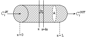 |
Fig. 1:Representation of a PFR filled with catalyst.
A. Steady state mass balance
If e is the bed porosity, the area, A, available for the catalyst particles is [(1-e) A] and the area available for the fluid is [e A]. Equation (A.1) becomes:
![]() (A.2)
(A.2)
where ji is the molar flux of component i, rb is the bulk density and ri is the rate of formation of component i.
Re-writing equation (A.2):
![]() (A.3)
(A.3)
![]() (A.4)
(A.4)
Considering a plug flow with axial dispersion, the molar flux is given by:
![]() (A.5)
(A.5)
where ui is the interstitial velocity of the fluid, Ci is the concentration of component i in the fluid and Dax is the axial dispersion coefficient.
![]() (A.6)
(A.6)
Normalizing some
of the variables: ![]() (L is the PFR length),
(L is the PFR length), ![]() (
(![]() where
where ![]() is the feed
concentration of component i),
is the feed
concentration of component i),
![]() (A.7)
(A.7)
dividing by ![]() , equation (A.7)
becomes:
, equation (A.7)
becomes:
![]() (A.8)
(A.8)
where Pe
is the dimensionless Peclet number given by ![]() , and t is the space-time given by
, and t is the space-time given by ![]() .
.
Grouping the
term ![]() as
a reaction term represented by
as
a reaction term represented by ![]() , the steady state mass balance of
component i becomes:
, the steady state mass balance of
component i becomes:
![]() (A.9)
(A.9)
 In the limiting case of absence
of dispersion
In the limiting case of absence
of dispersion ![]() , equation (A.9) becomes:
, equation (A.9) becomes:
![]() (A.10)
(A.10)
B. Steady state energy balance
![]() (B.2)
(B.2)
where jh is the heat flux, ![]() is the heat of
reaction j, rj is the rate of reaction j, Alat
is the lateral area of the volume element, U is the overall
heat-transfer coefficient, T is the reactor temperature and Tw
is the reactor wall temperature.
is the heat of
reaction j, rj is the rate of reaction j, Alat
is the lateral area of the volume element, U is the overall
heat-transfer coefficient, T is the reactor temperature and Tw
is the reactor wall temperature.
Re-writing equation (B.2):
![]() (B.3)
(B.3)
The heat flux can be given by:
![]() (B.4)
(B.4)
where r is the solution density and Cp is the solution heat capacity.
If R0 is the reactor radius, the lateral area of the volume element of length dz is:
![]() (B.5)
(B.5)
and its sectional area is:
![]() (B.6)
(B.6)
leading to:
![]() (B.7)
(B.7)
Substituting into equation (B.3):
![]() (B.8)
(B.8)
Normalizing the
space variable: ![]() , remembering the space-time
definition
, remembering the space-time
definition ![]() and
rearranging equation (B.8):
and
rearranging equation (B.8):
![]() (B.9)
(B.9)
The term ![]() is
dimensionless and is referred as NTU (number of heat transfer units).
is
dimensionless and is referred as NTU (number of heat transfer units).
Finally, the steady state energy balance becomes:
![]() (B.10)
(B.10)
C. Boundary Conditions
In the absence of dispersion, we only need one boundary condition:
 (C.1)
(C.1)
where T0 is the initial reactor temperature.
v Algorithm to solve the problem
We have a non-linear system of Ordinary Differential Equations (ODE) to solve:
 (1)
(1)
The program we developed uses subroutine DDASSL (Brenan et al., 1989) to solve this system. This code solves a system of differential/algebraic equations of the form delta(t, y, yprime)=0, with delta(i) = yprime(i) – y(i), using the backward differentiation formulas of orders one trough five. t is the current value of the independent variable (in our case t = X), y is the array that contains the solution components at t (in our case we have: y(i) = f(i), i=1,4 and y(5) = T) and yprime is the array that contains the derivatives of the solution components at t.
The program solves the system from t to tout and it is easy to continue the solution to get results at additional tout. In our case, we are going to get results at different values of X, between 0 and 1.
This problem is rather complex because most of the other variables depend on yi: the kinetic, adsorption and thermodynamic equilibrium “constants” depend on T (y5), the solution heat capacity and density also depend on T, the reaction rate and the components rate of formation depend on yi (fi (i=1,4) and T), as the activity coefficients.
In Figure 2 is the algorithm to solve our problem.
 |
Fig. 2: Algorithm to solve the problem.
Some results
For both cases, isothermal and non-isothermal, the feed concentrations were the same:

These concentrations lead to a feed mole ratio MeOH/isoamylenes, RM/IA, of 1.0.
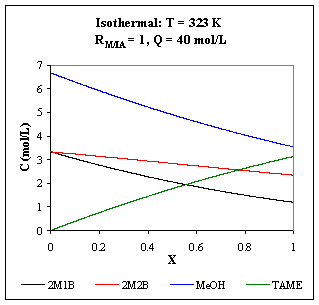 |
Fig. R.1: Concentration profiles for a 10 m3 isothermal PFR operating at 323 K.
Fig. R.2: Concentration profiles for a 10 m3 isothermal PFR operating at 343 K.
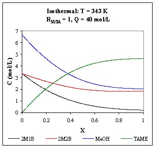
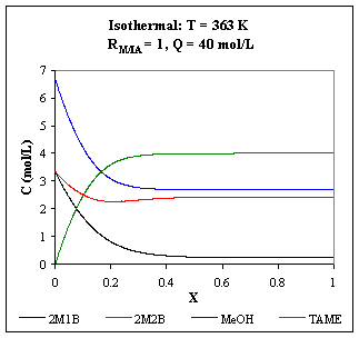
Fig. R.3: Concentration profiles for a 10 m3
isothermal PFR operating at 363 K
As the temperature increases, the reactions are faster, favoring TAME production, but the chemical equilibrium is moved to the opposite direction: for an operating temperature of 363 K, the equilibrium concentration of TAME is reached faster than for 343 K, but its value is lower.
b) Figure R.4 represents the exit concentrations as a function of the entering temperature, T0, for a 10 m3 isothermal PFR operating with a flow of 40 L/min.
Fig. R.4: Exit concentrations 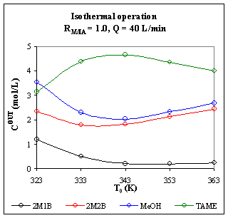
as function of T0,
for a 10 m3 isothermal PFR
Figure R.4 shows that there is an optimum operating temperature around 343 K that leads to a maximum exit concentration for TAME. It is due to the fact that we have a system with competition between kinetics and equilibrium, as we are going to see for the non-isothermal PFR
c) We chose a reactor diameter of 1 m (for a volume of 10 m3 it leads to a reactor length of 12.7 m approximately) and for the wall temperature, we decided to use room temperature: 298 K. The entering temperature is 353 K.
It is important to notice that the catalyst used in TAME production is a macroreticular strong cation ion-exchange resin in hydrogen form (Amberlyst 15 Wet, Rohm & Haas) that has a maximum operating temperature of 393 K.
Figure R.5 represents the concentration (a) and temperature (b) profiles for an operating flow of 200 L/min.
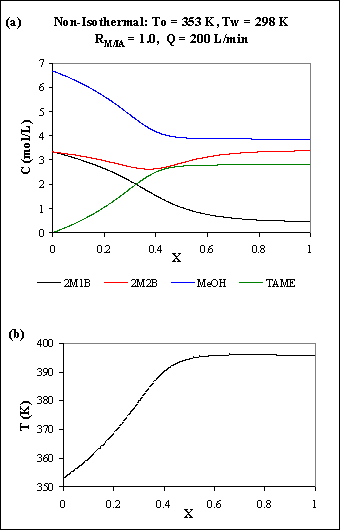
Fig. R.5: Non-isothermal PFR: (a)
concentration profiles; (b) temperature profile.
Figure R.5(a) shows the competition between the three reactions: first, 2M1B and 2M2B react with MeOH to produce TAME and the reactants concentrations decrease and TAME concentration increases; but then, although MeOH and TAME concentrations are almost constant, 2M1B is still decreasing and 2M2B starts to increase: the third reaction, the isomerization, is now more evident.
The temperature profile (Fig. R.5(b)) shows that the reactor seams to be almost adiabatic (no heat losses through the reactor walls) since the reactor temperature is always increasing. This close to adiabatic behavior was expected since the reactor diameter is rather large: 1 m. But the temperature reaches a value that is not convenient for the catalyst: remember that its maximum operating temperature is 393 K and the reactor is reaching almost 396 K.
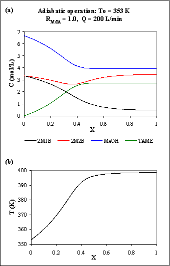
To see what is the maximum temperature that the reactor reaches, we can make it
adiabatic setting the overall heat-transfer coefficient equal to zero: U
= 0. In Figure R.6 are the results for the adiabatic reactor.
Fig. R.6: Adiabatic PFR: (a) concentration profiles; (b) temperature profile.
The maximum temperature reached by the reactor is 398.6 K. Comparing Figures R.5 and R.6 it is easy to see that the non-isothermal 1m diameter PFR can be considered adiabatic: the concentration and temperature profiles are almost the same.
To improve the
reactor production, i.e., to reach higher exit concentrations of TAME, we can
use a multi-tubular reactor. Lets think of a reactor composed of 4000 tubes
(each one considered as a PFR) with a diameter of 1’’ each. To have a total
reactor volume of 10 m3, each tube has a length of 5 m. In order to
compare the results of the multi-tubular reactor with the ones obtained with
the 1 m diameter PFR (Fig. R.5), we have to choose similar operating
conditions: to have a total operating flow of 200 L/min, the equivalent flow in
each tube is 0.05 L/min; since the reactor is now really cooled, we will choose
the “best” temperature for the cooling fluid (343 K, as seen with the
isothermal behavior runs). Figure R.7 shows the results 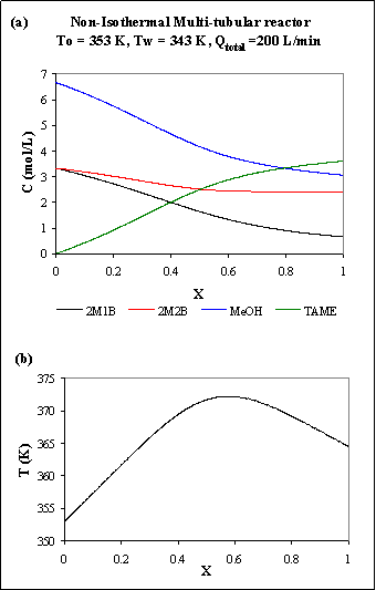
for one of this tubes operating in the above conditions.
Fig. R.6: Multi-tubular reactor: (a) concentration profiles; (b) temperature profile.
The maximum temperature reached is 373 K - in this case there are no problems with the catalyst - and the exit concentration of TAME is higher: 3.613 mol/L against 2.830 mol/L for the PFR in Figure R.5, which represents an increase of 27.7 %.
References
Brenan, K., Campbell, S. and L. Petzold, “Numerical Solution of Initial-Value Problems in Differential-Algebraic Equations, Elsevier, N.Y. (1989).
Kitchaiya, P. and R. Datta, “Ethers from Ethanol. 2. Reaction Equilibria of Simultaneous tert-amyl Ethyl Ether Synthesis and Isoamylene Isomerization”, Ind. Eng. Chem. Res. 34 (1995) 1092-1101.
Kiviranta-Pääkkönen, P.K., Struckman, L.K. and A.O.I. Krause, “Comparison of the Various Kinetic Models of TAME Formation by Simulation and Parameter Estimation”, Chem. Eng. Technol. 21 (1998) 321-326.
Oktar, N., Mürtezaoglu, K., Dogu, T. and Gülsen Dogu, “Dynamic Analysis of Adsorption Equilibrium and Rate Parameters of Reactants and Products in MTBE, ETBE and TAME Production”, Can.J. Chem. Eng. 77 (1999) 406-412.
Perry, R.H. and Dan W. Green, “Perry’s Chemical Engineers’ Handbook”, 7th edition, McGraw-Hill (1997).
Reid, R.C., Prausnitz, J.M. and Thomas K. Sherwood, “The Properties of Gases and Liquids”, 3rd edition, McGraw-Hill (1977).
Reid, R.C., Prausnitz, J.M. and B.E. Poling, “The Properties of Gases and Liquids”, 4th edition, McGraw-Hill (1987).
Vilarinho Ferreira, M.M. and J.M. Loureiro, “Synthesis of TAME: Kinetics in Batch Reactor and Thermodynamic Study”, presented on the “3rd European Congress of Chemical Engineering, ECCE3”, Nuremberg, Germany (June 2001).
Zhang, T. and R. Datta, “Integral Analysis of Methyl tert-Butyl Ether Synthesis Kinetics”, Ind. Eng. Chem. Res. 34 (1995) 730-740.


