The unsteady-state mole balance is given by Equation (4-46)
where we use shorthand notation:
A typical plot of CA vs. T for steady-state operation (i.e., MB = 0) is shown in Figure R9.4-1. For example, if the reaction is first-order and irreversible, the equation for the "MB = 0 curve" would be
Using the mole balance (MB = 0) to divide the phase plane
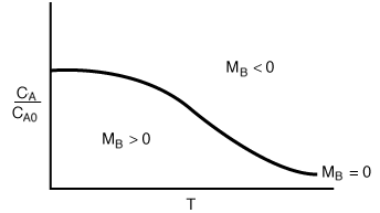
Regions of the Phase Plane
This curve (i.e., MB = 0) divides the phase plane into two regions:
where concentration increases with time, and
where concentration decreases with time.
We now consider the relative magnitude of two positive terms, ![]() When
When ![]() is positive and concentration increases with time. When
is positive and concentration increases with time. When![]() (i.e.
(i.e. ![]() ), the derivative is negative and the concentration decreases with time.
), the derivative is negative and the concentration decreases with time.
To continue our analysis of the approach to steady state we need to consider the energy balance next. For operation of a CSTR with![]() , the unsteady energy balance, Equation (9-11), can be rearranged in the form
, the unsteady energy balance, Equation (9-11), can be rearranged in the form
Unsteady
mole
balance
![]()
where ![]()
Figure R9.4-2 shows a typical plot of CA vs.T for EB = 0. For an irreversible first-order reaction, the equation for the "EB = 0 curve" would be

This curve divides the phase plane into two regions:
1.
where temperature increases with time, and
2.where temperature decreases with time.
Using the
energy balance (EB = 0) to divide the phase plane
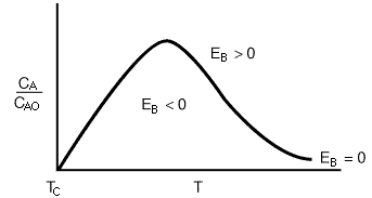
Figure R9.4-2
Regions of the Phase Plane
Temperature can either decrease or increase with time depending on the
relative magnitudes of ![]() and
and![]() .
.
Next we combine Figures R9.4-1 and R9.4-2 to yield Figure R9.4-3, which shows
the curve for MB = 0 and EB
= 0 for a particular set of parameter values (e.g.,![]() ).
).
(Note that other parameter values will give a different set of intersections of MB = 0 and EB = 0). The steady-state value is, of course, the intersection of the MBand EBcurves. We can divide the phase plane into four quadrants:
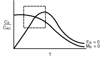
Figure R9.4-3
Regions of the Phase Plane

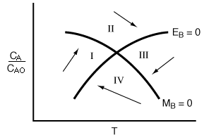
Figure R9.4-4
Quadrants of the phase plane.
The dashed square around the steady state in Figure R9.4-3 is expanded and shown in Figure R9.4-4 identifying the various quadrants. Temperature is increasing in quadrants I and II and decreasing in quadrants III and IV, while the concentration of species A is increasing in quadrants I and IV and decreasing in II and III. With this information we may make qualitative sketches of the temperature-concentration pathways or trajectories.
Figure R9.4-4 shows a sketch of two different approaches to the steady state that result from starting the reactor up at the same initial temperature, Ti but at two different initial concentrations. Starting at Ti and CA = 0 in quadrant IV, we know that CA, will increase and T will decrease until we cross the solid line of the EB = 0 curve into quadrant I, where both CA and T increase until we cross the MB = 0 curve into quadrant II, where CA decreases and T increases. The CA vs.T phase-plot trajectory continues its spiral approach to the steady state(CAs,Ts) as it crosses into quadrant III, where both CA and T decreases and then it reenters quadrant IV. This trajectory is shown in Figure R9.4-5. A similar type of reasoning can be used to trace out the trajectory starting at Ti and CAi.
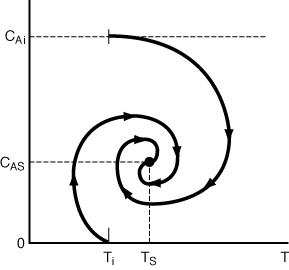
Figure R9.4-5
Approach to the steady state.
Example CD13-2
Startup of a CSTR
Falling Off the Steady State
Proportional-Integral (PI) Control