
Monte
Carlo Simulation of Single Molecule Kinetics
The following two Mathematica programs
can be used to simulate single-molecule data sets for systems that
interconvert between two distinct states, i.e. fluorescent on-state and
non-fluorescent off-state.
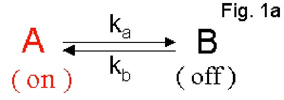
The One-conformation Model program simulates single-molecule data for a
simple first-order reaction shown in Fig. 1a. The molecule leaves state
A for state B with a forward rate, ka, and it converts back to state A
with a backward reaction rate, kb. State A and B are assumed to be
distinguishable spectroscopically in single-molecule experiments, i.e.
state A is fluorescent (on) and state B is non-fluorescent (off). The
program generates both single-molecule fluorescence traces and dwell
times that the system resides in the two fluorescent states (on-times
and off-times).
There are four input parameters that can be changed in the program,
including step, Prob, Turnover and Time.
1) step: it determines the time resolution and is regarded as the unit
time in the simulation. step = 0.01 means the program generates data
every 0.01 second.
2) Prob: it’s a 2¥1 vector. Prob[1] = 1 - exp(-kb*step) is the
probability of the molecule leaving the off-state; Prob[2] =1 -
exp(-ka*step) is the probability of leaving the on-state. When the step
size is small so that ka*step and kb*step are small, Prob[1] = kb*step
and Prob[2] = ka*step. For example, if kb = 2 s-1, ka = 3 s-1 and step
= 0.01 s, Prob[1] = 0.02 and Prob[2] = 0.03.
3) Turnover: this parameter determines the total number of turnover to
be generated in the simulation. One can set this number depending on
the desired number of on-times and off-times, which is also the number
of turnovers, to be generated from the program.
4) Time: it defines the total number of data points and the length of
the single molecule trace to be generated. For example, if Time =
10000, with a step size of 0.01 second, the length of the single
molecule trace is 100 seconds (Time * step). One can roughly estimate
this parameter from the number of turnovers to be generated and the
forward as well as backward reaction rates, or simply put in a fairly
large value.
In the end, the simulated single molecule fluorescence trace is
exported to “C:\\simulation\\data\\one-conform.dat” and the on-times as
well as off-times are exported to
“C:\\simulation\\data\\on-conform-on-off.dat”. The output locations can
be changed.
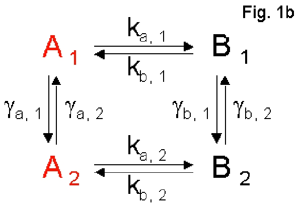
The Two-conformation Model program simulates single-molecule data for
systems that involve a conformational fluctuation that results in
reaction rates randomly switching between distinct values as shown in
Fig. 1b. In conformation 1, the system turns over between the
fluorescent on-state, A1, and non-fluorescent off-state, B1, with
reaction rate, ka, 1 and kb, 1, respectively. In conformation 2, the
system turns over between the fluorescent on-state, A2, and
non-fluorescent off-state, B2, with different reaction rates, ka, 2 and
kb, 2, respectively. The two on-states, A1 and A2, are fluorescently
indistinguishable, so as the two off-states, B1 and B2. The two
conformations can interconvert between each other with different rates,
ga,i and gb,i (i = 1, 2). The program generates single-molecule data,
including single-molecule fluorescence trajectories, dwell times that
the system resides in the two fluorescent states (on-times and
off-times), conformation trajectories, and dwell times that the system
resides in the two conformation states.
There are five input parameters that can be changed
in the program, including step, Prob, cProb, Turnover and Time.
1) step: it determines the time resolution and is regarded as the unit
time in the simulation. step = 0.01 means the program generates data
every 0.01 second.
2) Prob: it’s a 2¥2 matrix, describing the probability of leaving a
specific state. In the above two-conformation model, there are 4
possible microscopic states, including fluorescent states A1 & A2,
and non-fluorescent states B1 & B2. Prob[i, 1] = 1 - exp(-(kb,i +
gb,i)*step) is the probability of leaving the non-fluorescent state,
Bi, in conformation i (i = 1, 2); Prob[i, 2] = 1 - exp(-(ka,i +
ga,i)*step) is the probability of leaving the fluorescent states, Ai,
in conformation i. When the step size is very small, Prob[i, 1] = (kb,i
+ gb,i)*step and Prob[i, 2] = (ka,i + ga,i)*step. For example, when
kb,1 = ka,1 = 1 s-1, kb,2 = ka,2 = 5 s-1, and gb,1 = ga,1 = gb,2 = ga,2
= 0.3 s-1, Prob[1, 1] = 0.013, Prob[1, 2] = 0.013, Prob[2, 1] = 0.053,
and Prob[2, 2] = 0.053.
3) cProb: it’s a 2¥2 matrix, describing the probability of the
system converting into a different conformation state, not a different
fluorescent state, given that it is leaving a specific state.
Therefore, cProb[i, 1] = gb,i /(kb,i + gb,i) is the probability of
interconversion between the two non-fluorescent states Bi, and cProb[i,
2] = ga,i /(ka,i + ga,i) (i =1, 2) is the probability of
interconversion between the two fluorescent states Ai. For example,
when kb,1 = ka,1 = 1 s-1, kb,2 = ka,2 = 5 s-1, and gb,1 = ga,1 = gb,2 =
ga,2 = 0.3 s-1, cProb[1, 1] = 0.2308; cProb[1, 2] = 0.2308, cProb[2, 1]
= 0.0566, and cProb[2, 2] = 0.0566.
4) Turnover: this parameter determines the total number of turnover to
be generated in the simulation. One can set this number depending on
the desired number of on-times and off-times, which is also the number
of turnovers, to be generated from the program.
5) Time: it defines the total number of data points and the length of
the single molecule trace to be generated. For example, if Time =
10000, with a step size of 0.01 second, the length of the single
molecule trace is 100 seconds (Time * step). One can roughly estimate
this parameter from the number of turnovers to be generated and the
forward as well as backward reaction rates, or simply put in a fairly
large value.
In the end, the simulated single molecule fluorescence trace is
exported to “C:\\simulation\\data\\trace.dat”; the on-times as well as
off-times are exported to “C:\\simulation\\data\\on-off.dat”; the time
evolution of the conformational state of the system is exported to
“C:\\simulation\\data\\conf-trace.dat”; and the time durations that the
system resides in the two conformational states are exported to
C:\\simulation\\data\\c1-c2.dat”. The output locations can be changed.
Mathematica files;
one-conformation.nb
two-conformation

Main Page
People
Current Research
Facilities
Publications
Links