By Shiming Duan, Last Update: 8/13/2010 5:01 PM
IV. Controllability and Observability of Systems of DDEs
In Chapter 2 and Chapter 3, analytical solutions for systems of DDEs have been derived. These results are extended in this chapter to investigate the point-wise controllability and observability and their Gramians for linear time-delay systems.
Again, consider the system of DDEs in matrix-vector form:

where ![]() and
and ![]() are
are
![]() coefficient matrices,
coefficient matrices, ![]() are
are ![]() coefficient
matrices,
coefficient
matrices, ![]() is an
is an ![]() state
vector,
state
vector, ![]() is an
is an ![]() input
vector,
input
vector, ![]() is an
is an ![]() preshape
function, t is time, and h is a constant scalar time
delay. The coefficient matrix C
is
preshape
function, t is time, and h is a constant scalar time
delay. The coefficient matrix C
is ![]() and y(t) is a
and y(t) is a ![]() measured output vector.
measured output vector.
Point-wise Controllability
The system of DDEs is point-wise controllable if, for any given initial conditions g(t) and x0, there exists a time t1, 0 < t1 < ![]() , and an admissible (i.e., measurable and bounded on a
finite time interval) control segment u(t) for
, and an admissible (i.e., measurable and bounded on a
finite time interval) control segment u(t) for ![]() such that
x(t1; g, x0, u(t)) = 0 (Weiss,1967).
such that
x(t1; g, x0, u(t)) = 0 (Weiss,1967).
The following three sufficient and necessary conditions for point-wise controllability of systems of DDEs are equivalent.
The system of DDEs is point-wise controllable if and only if :
*

where ![]() is
the controllability Gramian of the system of DDEs
is
the controllability Gramian of the system of DDEs
* All rows of
![]()
are linearly independent on ![]() .
.
* All rows of
![]()
are linearly independent over the field of complex number except at the roots of the characteristic equations of system of DDEs.
Point-wise Observability
The system of DDEs is point-wise observable in [0, t1] if the initial point x0 can be uniquely determined from the knowledge of u(t), g(t), and y(t) (Delfour and Mitter, 1972).
The following three sufficient and necessary conditions for point-wise observability of systems of DDEs are equivalent.
The system of DDEs is point-wise observable if and only if:
*

where ![]() is
the observability Gramian of the system of DDEs
is
the observability Gramian of the system of DDEs
* All rows of
![]()
are linearly independent on ![]() .
.
* All rows of
![]()
are linearly independent over the field of complex number except at the roots of the characteristic equations of system of DDEs.
Example 4.1: Consider the following second-order time-delay systems:

![]()
where x1, x2 are the two states of the system, h is the time delay, u is the input and c1, c2 are the parameters for matrix Ad. In this example, we will investigate the controllability of the system for different values of c1,and c2:
Case 1: c1= c2 =0
Case 2: c1=0.1, c2 =0
Case 3: c1=0, c2 =0.1
Case 1: when c1= c2 =0, the system of DDEs will resort to a system of ODEs:

One can verify that the system is uncontrollable by checking the rank of the controllability matrix:
![]()
Thus, the system of ODEs is not controllable.
Case 2: When c1=0.1, c2 =0, the system becomes

One can
calculate the controllability
Gramian of the system of DDEs
using the approach introduced in this chapter. First, we can use similar
approach introduced in Ex. 3.1 to obtain ![]() and
and ![]() for the system of DDEs.
for the system of DDEs.
|
Index j |
Eigenvalue |
Coefficient |
|
1 |
-0.7815 |
|
|
2 |
-2 |
|
|
3 |
-3.9173+4.0932i |
|
|
4 |
-3.9173-4.0932i |
|
|
5 |
-4.7267+10.6592i |
|
|
6 |
-4.7267-10.6592i |
|
|
7 |
-5.1671+17.0389i |
|
|
8 |
-5.1671-17.0389i |
|
|
9 |
-5.4721+23.3729i |
|
|
10 |
-5.4721-23.3729i |
|
Second, we evaluate controllability Gramian of the system of DDEs

Here, we pick t1=4. Please note that the result of controllability does not depend on the selection of t1 since the sytem is linear. From Fig.4.1, we can see that controllability Gramian does not have full rank even more branches are considered. Thus, the system is not point-wise controllable by checking the rank of the controllability Gramian.
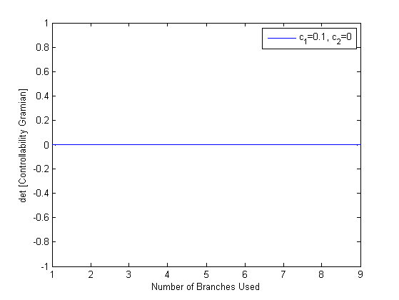
Fig. 4.1 Determinant of controllability Gramian for Case 2 in Ex.4.1.
The value of determinant is a constant zero when more branches are used.
Case 3: When c1=0, c2 =0.1, again, one can use Gramian to check the controllability.

Again,
we obtain ![]() and
and ![]() for the system of DDEs first.
for the system of DDEs first.
|
Index j |
Eigenvalue |
Coefficient |
|
1 |
-0.8108 |
|
|
2 |
-3.0086 |
|
|
3 |
-4.4064+1.0364i |
|
|
4 |
-4.4064-1.0364i |
|
|
5 |
-6.8827+8.2735i |
|
|
6 |
-6.8827-8.2735i |
|
|
7 |
-7.8740+14.9002i |
|
|
8 |
-7.8740-14.9002i |
|
|
9 |
-8.5284+21.3555i |
|
|
10 |
-8.5284-21.3555i |
|
Here, we pick t1=4 and calculate the obser Gramian.
In Fig.4.2, we can see that the determinant of the controllability Gramian converges to non-zero values. Thus, the controllability Gramian has full rank and the system is point-wise controllable.

Fig. 4.2 Determinant of controllability Gramian for Case 3 in Ex.4.1.
The value of determinant converges to a non-zero value as more branches are considered.
Example 4.2: Consider the closed-loop pendulum control system discussed in Ex.3.1.
It is assumed that only the angular velocity of the pendulum is measured and
the control is a velocity feedback control  .
In this example, if only the velocity is measured, we want to know whether we
can
.
In this example, if only the velocity is measured, we want to know whether we
can
reconstruct the other state, the angular position, from the measurements. In other words, we want to check whether the closed-loop time delay system is point-wise observerable.

The
procedure here is quite similar to the procedure introduced in Ex.4.1. First, we obtain ![]() and
and ![]() for the system of DDEs.
for the system of DDEs.
|
Index j |
Eigenvalue |
Multiplicity of |
Coefficient |
|
1 |
|
1 |
|
|
2 |
|
1 |
|
|
3 |
|
1 |
|
|
4 |
|
1 |
|
|
5 |
|
1 |
|
|
6 |
|
1 |
|
|
7 |
|
1 |
|
|
8 |
|
1 |
|
Then, we pick t1=4 and calculate the observability Gramian.

In Fig.4.3, we can see that the determinant of the observability Gramian converges to non-zero values. Thus, the observability Gramian has full rank and the system is point-wise observable.
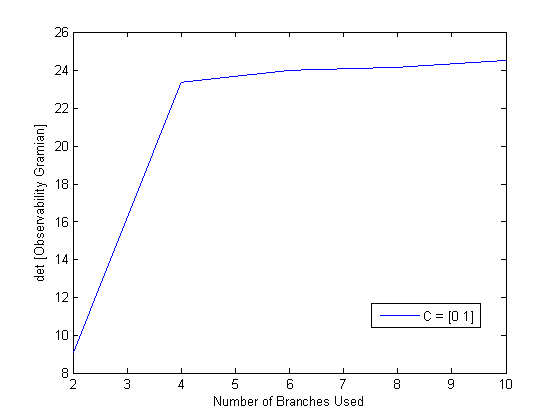
Fig. 4.3 Determinant of observability Gramian of the system in Ex.4.2.
The value of determinant converges to a non-zero value as more branches are considered.