By Shiming Duan,  Last Update: 8/13/2010 5:10 PM

VII. Design of Observer-Based Feedback Control for Time-Delay Systems

In Chapter 4, the problem of the controllability and observerability of systems of DDEs was investigated. In Chapter 5 and Chapter 6, the feedback control problem for time-delay systems was solved using the Lambert W function approach. One assumption we made during the design procedure is that all states are measurable. However, in many engineering applications, due to cost and difficulties in sensor implementation, some states are not directly measured. Thus, to realize the proposed state feedback control scheme, a state estimator, or observer,  is necessary. In this chapter, we demonstrate the design of observers for systems of DDEs, together with the feedback control synthesis of the closed-loop systems.

Problem Formulation

Consider a linear time-invariant (LTI) system of DDEs with a single constant time-delay

The state feedback control, together with a reference input, , can be written as

If the states,, are not measured, one must reconstruct the states from the available measurements, , and use the estimated states, , in the controller.

Observer-Based Feedback Design

The procedure of designing an observer-based feedback control for a system of DDEs can be summarized as follows:

Step 1: Obtain the equations for the closed-loop system

where .  Choose the desired rightmost eigenvalues for the closed-loop system based on time-domain specifications (See Chapter 6).

Step 2: Select proper gains and  to place the rightmost poles at desired places in the s-plane following the approach introduced in Chapter 5. If a solution cannot be found, one should go back to step 1 and either pick other desired rightmost eigenvalues, or try with fewer desired eigenvalues, or place the real parts only.

Step 3: Design an observer with a gain L:

where . Thus, the dynamics of the state error can be described as

Then choose the desired rightmost eigenvalues for the observer. A typical rule of thumb is to make the dynamics of the observer 1.5~2 times faster than the dynamics of the plant.

Step 4: Select a proper gain L to place the rightmost eigenvalues of the observer at the desired location. If not successful, one should go back to step 3 and make a different selection of the desired observer eigenvalues.

Separation principle

It can be shown that the the eigenvalues of the observer are not affected by feedback:

It can be shown that

which further leads to

Thus, the design of gains and for the controller and the selection of L for the observer can be done independently.

Note there is a typo in Eq.7.5 and Eq.7.6 in the book. Please refer to the above corrected equations for your use.

Example 7.1 Pendulum System (Observer-Based Feedback Control)

Consider the feedback control problem in Ex. 5.2 for the linearized pendulum system

where . In this example, we consider the design of an observer-based full state feedback control for the system assuming only the angular position is measured.

Step 1: Note that the closed-loop system with the feedback  can be written as

where

First, one can verify that the system is point-wise controllable by calculating the controllability Gramian of the system (e.g., see Ex.4.1). Then, the desired rightmost eigenvalues for this closed-loop system are selected based on time-domain specifications (see Ex. 6.2). Here we pick the desired rightmost eigenvalues to be .

Step 2: Select a proper gain  to place the rightmost poles of the plant at the desired location () in the s-plane. Following the results in Ex.6.2, we obtain .

Step 3: One can verify that the system is point-wise observable by calculating the observabilityGramian of the system (e.g., see Ex.4.2). After that, design an observer with a gain L

where . Since the rightmost poles of the plant are , we select the poles of the observer to be . Thus, the dynamics of the observer will be 3 times faster than the dynamics of the plant.

Step 4: Using the function place in Matlab, we obtain . Note that since  for the plant in this example, the observer system becomes a system of ODEs. Thus, one can directly apply the techniques for ODEs to select the gain L. However, in general, the observer will be a system of DDEs and one should use the Lambert W function approach for assigning the rightmost eigenvalues of the observer.

The simulation results are shown in the following two figures. The free reponse with initial conditions [1; 1]^T is plotted in Fig.7.1. In Fig.7.2, it shows the forced response of the system under a sine input u=sin(t).  Both results show that the estimated states converge to the actual states fastly.

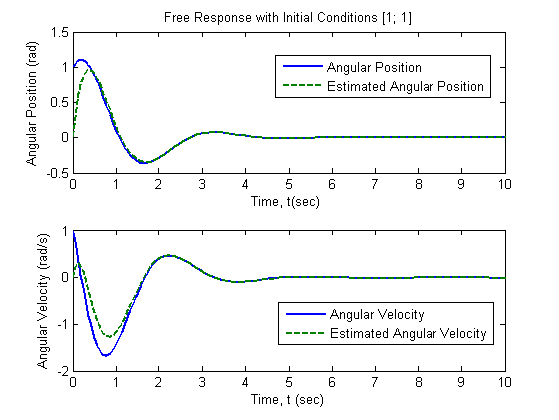
Fig.7.1 Free response of the closed-loop observer-based feedback control system

Fig.7.2 Forced response of the closed-loop observer-based feedback control system

Example 7.2 Observer Design for Human Immunodeficiency Virus (HIV) Pathogenesis Model

As introduced in Ex. 1.3, the HIV pathogenesis can be modeled via the following delay differential equations (Nelson et al., 2000). 

where t is the elapsed time since the treatment is initiated, h is time-delay, T₀ is the target T-cell concentration, T^* is the concentration of productively infected T-cell, V_I  is the concentration of infectious virions in the plasma, V_NI  is the concentration of non-infectious virions in the plasma, c is rate of virion clearance,  is the rate of loss of the virus-producing cell, N is the mean number of new virions produced per infected cell during its lifetime, and n_p represents the drug efficacy of a protease inhibtor. It is assumed that HIV infects targeted cells with a rate and causes them to become productively infected T-cells, T^*. The values of the parameters are the same as in Ex.1.3.

The problem for this example is that, in practice,  V_I  and V_NI  cannot be directly measured. The total virion concentration, i.e., V_I +V_NI , is the measurable variable from experiments. Therefore, we want to estimate the states V_I  and V_NI  using an observer.

Note that the system can be written as a matrix DDE

where

and 

First, check the observability of the system using the Lambert W function approach. Instead of calculating the gramian, here we use the conditions in Eqn.4.1 in the book to test for controllability

To prove that ,  and are linearly independent, we need to show the existence of scalars p_1, p_2, p_3, such that

Using the following Matlab script, for the paramtere values given there,  and selecting  p₁=1, p₂=3, p₃=5 yields rank =3 and completes the observerbility test. Since the system is observable, we can design an observer to estimate the states.

------------Matlab Code---------------

syms s

T = 0.91;m=0;T0=408000;N=480;np=0.70;c=4.3;delta=1.57;k=c/(N*T0);  %

A=[-delta 0 0;(1-np)*N*delta -c 0;np*N*delta 0 -c]                % Coefficients in state-space forms

Ad=[0 k*T0*exp(-m*T) 0;0 0 0;0 0 0]

C = [0 1 1];

char = s*eye(3)-A-Ad*exp(-s*T)

obs_gram = C*char^-1;

c1 = subs(obs_gram, 1); % p1 =1

c2 = subs(obs_gram, 3); % p2 =3

c3 = subs(obs_gram, 5); % p3 =5

rank([c1;c2;c3])

------------End---------------

Next we design an observer with a gain L:

where . Thus, the dynamics of the state error can be described as

The rightmost eigenvalue of the plant is found to be  −0.61. To make the dynamics of the observer fast enough with specified parameters, we place the rightmost eigenvalue of the observer to be −0.6*2.5 = −1.5.  Using the introduced eigenvalue assignment approach (e.g., see Ex.6.2), we obtain

which places the eigenvalues of the principal branch at

The simulation results for the free response with initial conditions [10⁵; 10⁵; 10⁵]^T are plotted in Fig.7.3 showing the fast convergence of the observer states to the plant states.

Fig.7.3 Free response of the observer system of the HIV model