Table 1: Types of local federal expenditure
|
variable | description |
|
transfer payments | transfer payments to individuals |
|
civilian employment | Federal government civilian employment |
|
military employment | Federal government military employment |
|
civilian salaries | salaries and wages, all civilian and Postal Service employees |
|
military salaries | salaries and wages, all military personnel |
|
civilian procurements | procurement contracts, all except Defense Department |
|
military procurements | procurement contracts, Defense Department |
|
direct payments | direct payments other than for individuals |
|
education transfers | transfers to local governments for education |
|
highways transfers | transfers to local governments for highways |
|
social welfare transfers | transfers to local governments for public welfare, employment security, health and hospitals, housing |
|
other transfers | all other transfers to local governments |
Notes:
![]() All variables are used per capita, based on county population
All variables are used per capita, based on county population ![]() .
.
![]() source, Bureau of Economic Analysis 1990.
source, Bureau of Economic Analysis 1990.
![]() source, Bureau of the Census 1984-90.
source, Bureau of the Census 1984-90.
![]() source, Bureau of the Census 1986-91 and 1991; county totals are
estimated as in Mebane 1993.
source, Bureau of the Census 1986-91 and 1991; county totals are
estimated as in Mebane 1993.
![]() units, $1000 per person.
units, $1000 per person.
![]() units, jobs per person.
units, jobs per person.
Table 2: 95% confidence intervals for support values that maximize local federal expenditures
| pre-midterm | ||||
| maximum is an elite-oriented targeting value | maximum is not in the elite-oriented range | |||
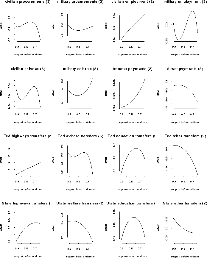
| civilian procurements | (.59, .61) | military procurements | (.00, 1.00) | |
| military employment | (.70, .71) | civilian employment | (.00, 1.00) | |
| civilian salaries | (.68, .68) | military salaries | no max | |
| Federal welfare transfers | (.61, .62) | transfer payments | no max | |
| Federal education transfers | (.60, .63) | direct payments | (.35, .44) | |
| State highways transfers | (.69, .75) | Federal highways transfers | (.00, 1.00) | |
| State education transfers | (.55, .59) | Federal other transfers | (.27, .37) | |
| State welfare transfers | (.35, .39) | |||
| State other transfers | no max | |||
| post-midterm | ||||
| maximum is an elite-oriented targeting value | maximum is not in the elite-oriented range | |||
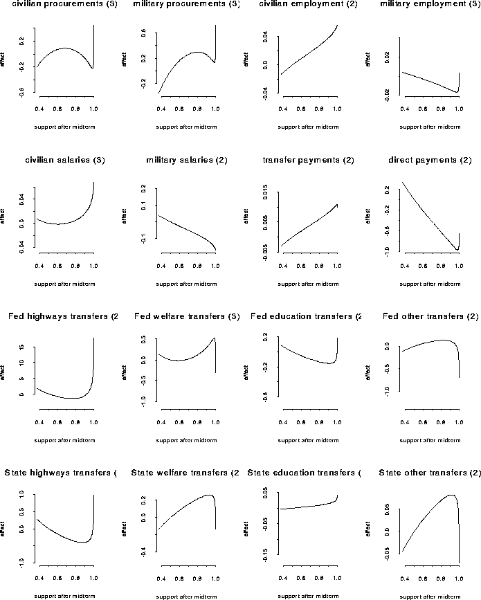
| civilian procurements | (.64, .71) | military procurements | (.79, .81) | |
| civilian employment | (.49, 1.00) | |||
| military employment | (.00, 1.00) | |||
| civilian salaries | (.02, 1.00) | |||
| military salaries | no max | |||
| transfer payments | (.00, 1.00) | |||
| direct payments | no max | |||
| Federal highways transfers | no max | |||
| Federal welfare transfers | (.98, .98) | |||
| Federal education transfers | no max | |||
| Federal other transfers | (.70, .91) | |||
| State highways transfers | no max | |||
| State welfare transfers | (.92, .94) | |||
| State education transfers | no max | |||
| State other transfers | (.74, .98) | |||
Source: Confidence intervals are computed using normal approximations and
asymptotic standard errors obtained by the delta method from the standard
errors of the coefficient estimates of the targeting polynomials.
![]() The polynomial does not have any maximum values.
The polynomial does not have any maximum values.
Table 3: 95% confidence intervals for support values that maximize changes in local federal expenditures
| institutionally less complex LFEs | ||||
| maximum is a voter-oriented targeting value | maximum is not in the voter-oriented range | |||
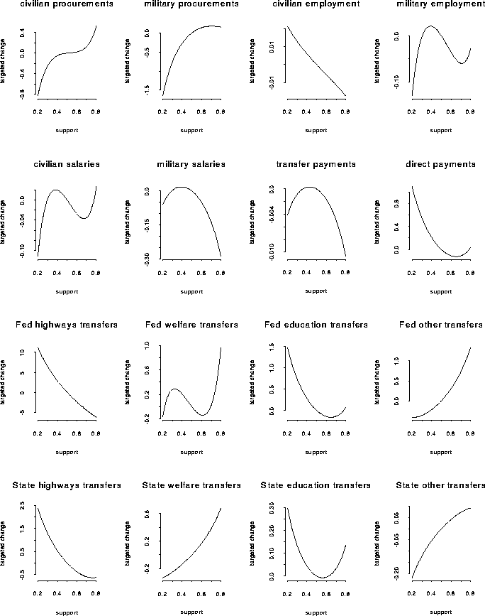
| military employment | (.38, .39) | civilian procurements | no max | |
| civilian salaries | (.37, .39) | military procurements | (.61, .79) | |
| military salaries | (.25, .55) | civilian employment | no max | |
| transfer payments | (.15, .75) | direct payments | no max | |
| institutionally complex LFEs | ||||
| maximum is a voter-oriented targeting value | maximum is not in the voter-oriented range | |||
| Federal welfare transfers | (.29, .35) | Federal highways transfers | no max | |
| Federal education transfers | no max | |||
| Federal other transfers | no max | |||
| State highways transfers | no max | |||
| State welfare transfers | no max | |||
| State education transfers | no max | |||
| State other transfers | (.00, 1.00) | |||
Source: Confidence intervals are computed using normal approximations and
asymptotic standard errors obtained by the delta method from the standard
errors of the coefficient estimates of the targeting polynomials.
![]() The polynomial does not have any maximum values.
The polynomial does not have any maximum values.
Table 4: Presidential vote choice probit regression equation estimates
| variable | I | II | III |
| Constant | -.252 | -.313 | -.318 |
| (-.509, .001) | (-.580, -.055) | (-.581, -.063) | |
|
Party identification | .521 | .534 | .533 |
| (.467, .581) | (.478, .595) | (.478, 594) | |
|
Spending scale | .440 | .524 | .381 |
| (.106, .778) | (.053, .718) | (.046, 715) | |
|
National economy evaluations | .540 | .524 | .526 |
| (.220, .874) | (.208, .866) | (.210, .870) | |
|
Family finances evaluations | .330 | .330 | .327 |
| (.060, .607) | (.057, .611) | (.059, .608) | |
|
Civilian employment | -- | 1.072 | .853 |
| (-.250, 2.401) | (.155, 1.570) | ||
|
Military employment | -- | .733 | .853 |
| (-.435, 1.885) | (.155, 1.570) | ||
|
Nongovernmental employment | 2.762 | 3.571 | 3.716 |
| (.351, 5.328) | (.960, 6.708) | (1.124, 6.848) | |
|
| 731.94 | 723.86 | 724.06 |
Source: Equations for the probability of voting for the Republican rather
than the Democratic presidential candidate, using 1988 ANES and contextual
data. N = 975 respondents from 91 counties. In equation I, 85.6%
correctly classified, ![]() .
. ![]() In equation II, 85.0% correctly
classified,
In equation II, 85.0% correctly
classified, ![]() . In equation III, 85.1% correctly classified,
. In equation III, 85.1% correctly classified,
![]() . Coefficients are probit MLEs. 95% confidence intervals
(percentile-t bootstrap) are in parentheses. Intercept-only:
. Coefficients are probit MLEs. 95% confidence intervals
(percentile-t bootstrap) are in parentheses. Intercept-only:
![]() log-likelihood = 1348.76.
log-likelihood = 1348.76.
![]() survey attitude variable.
survey attitude variable.
![]() county-level change (purged): total for 1987-88 minus total for 1985-86.
county-level change (purged): total for 1987-88 minus total for 1985-86.
![]() parameters constrained to equal one another.
parameters constrained to equal one another.
![]()
![]() (Goodman-Kruskal gamma) measures the rank correlation between
observed responses and predicted probabilities.
(Goodman-Kruskal gamma) measures the rank correlation between
observed responses and predicted probabilities.
Table 5: Probabilities of a pro-incumbent (pro-Republican) vote at minimum and maximum values of local-area employment changes and subjective economic evaluations
| national | family | |||||||||
| nongovernmental | civilian | military | economy | finances | ||||||
| employment | employment | employment | evaluations | evaluations | ||||||
| | | | | | | | | | | |
| at mean of PID | .35 | .71 | .39 | .63 | .36 | .61 | .43 | .64 | .45 | .58 |
| strong Democrat | .03 | .18 | .04 | .13 | .03 | .12 | .05 | .14 | .06 | .10 |
| Democrat | .09 | .36 | .11 | .28 | .10 | .26 | .14 | .28 | .15 | .23 |
| independent-Democrat | .22 | .57 | .25 | .47 | .23 | .46 | .29 | .49 | .30 | .42 |
| independent | .40 | .76 | .44 | .68 | .42 | .67 | .49 | .69 | .50 | .63 |
| independent-Republican | .61 | .89 | .65 | .84 | .63 | .83 | .69 | .85 | .71 | .81 |
| Republican | .79 | .96 | .82 | .94 | .80 | .93 | .85 | .94 | .86 | .92 |
| Strong Republican | .91 | .99 | .93 | .98 | .92 | .98 | .94 | .98 | .95 | .97 |
|
mean probability | .43 | .65 | .46 | .60 | .44 | .59 | .49 | .60 | .50 | .56 |
Source: Computed using the vote choice probit regression equation
point estimates of Table 4. The probability for each level of
party ID and each minimum or maximum value is computed with the other
variables in the equation at their mean values in the 1988 ANES sample.
Employment-changes values are for the purged data.
![]() Minimum value. For evaluations, 0 means ``worse.''
Minimum value. For evaluations, 0 means ``worse.''
![]() Maximum value. For evaluations, 1 means ``better.''
Maximum value. For evaluations, 1 means ``better.''
![]() Average of the probabilities over the seven party ID categories,
weighting by the sample proportions for the PID categories among voters in the
ANES data. In order from strong Democrat through strong Republican the
proportions are .199, .165, .112, .063, .128, .148, .186.
Average of the probabilities over the seven party ID categories,
weighting by the sample proportions for the PID categories among voters in the
ANES data. In order from strong Democrat through strong Republican the
proportions are .199, .165, .112, .063, .128, .148, .186.
Table 6: Effects of LFEs on individuals' subjective economic evaluations
| national economy | family finances | |
| variable | evaluations | evaluations |
| Intercept 1 | -.956 | -.628 |
| (.069) | (.090) | |
| Intercept 2 | .468 | .328 |
| (.065) | (.089) | |
|
Party identification | .166 | .111 |
| (.017) | (.019) | |
|
Family income in 1987 ($1000) | -- | .010 |
| (.0019) | ||
|
Military procurements | .126 | -- |
| (.064) | ||
|
Direct payments | -- | -.143 |
| (.066) | ||
|
Federal education transfers | -- | 6.492 |
| (3.264) | ||
|
Federal social welfare transfers | -1.843 | -- |
| (.440) | ||
|
Federal social welfare transfers | -2.442 | -- |
| (1.169) | ||
|
Civilian or military employment | -- | 35.15 |
| (17.95) | ||
|
Civilian or military employment | -91.46 | -- |
| (43.05) | ||
|
Nongovernmental employment | 3.722 | 2.900 |
| (1.286) | (1.393) |
Source: Ordered probit regression equations for the probability of giving a
more favorable response, using 1988 ANES and contextual data. National
economy N = 975 ( ![]() )
) ![]() and family finances N = 901
(
and family finances N = 901
( ![]() ) respondents. Coefficients are MLEs. Standard errors are in
parentheses.
) respondents. Coefficients are MLEs. Standard errors are in
parentheses.
![]() survey attitude variable.
survey attitude variable.
![]() county-level change: total for 1987-88 minus total for 1985-86.
county-level change: total for 1987-88 minus total for 1985-86.
![]()
![]() (Goodman-Kruskal gamma) measures the rank correlation between
observed responses and predicted probabilities.
(Goodman-Kruskal gamma) measures the rank correlation between
observed responses and predicted probabilities.
Table 7: Probabilities of evaluating the national economy as ``better'' at minimum and maximum values of the LFE changes that have heterogeneous effects
| social welfare | civilian | military | ||||
| transfers | employment | employment | ||||
| SPEND value | | | | | | |
| increase all index items | .067 | .298 | .029 | .389 | .011 | .349 |
|
neutral ( | .848 | .026 | .190 | .190 | .192 | .192 |
| decrease all index items | .9998 | .0004 | .552 | .070 | .709 | .087 |
Source: Computed using the ordered probit regression equation point estimates
of Table 6. The probability for each level of SPEND and each
minimum or maximum value is computed with the other variables in the equation
at their mean values in the 1988 ANES sample. LFE-changes values are for
unpurged data.
![]() Minimum value.
Minimum value.
![]() Maximum value.
Maximum value.
Table 8: Effects of LFEs on individuals' partisanship and spending tastes
| variable | party identification | spending scale |
| Intercept | -1.854 | -.278 |
| (.300) | (.019) | |
|
Family income in 1987 ($1000, logged) | .371 | -- |
| (.085) | ||
|
Direct payments | 1.121 | .170 |
| (.291) | (.037) | |
|
Federal education transfers | -15.22 | -- |
| (6.33) | ||
|
Federal highways transfers | -- | -.981 |
| (.520) | ||
|
Federal social welfare transfers | -2.065 | -- |
| (.747) | ||
|
Federal other transfers | 5.832 | .482 |
| (1.638) | (.193) | |
|
Nongovernmental employment | -- | .891 |
| (.357) | ||
|
Nongovernmental income | .161 | -- |
| (.055) |
Source: Ordinary least squares regression equations, using 1988 ANES and
contextual data. N = 901. Party identification equation residual mean
square error = 4.71 ( ![]() ). Spending scale equation residual mean
square error = .084 (
). Spending scale equation residual mean
square error = .084 ( ![]() ). Standard errors are in parentheses.
). Standard errors are in parentheses.
![]() survey attitude variable.
survey attitude variable.
![]() county-level change: total for 1987-88 minus total for 1985-86.
county-level change: total for 1987-88 minus total for 1985-86.
Figure 1: Effects of support on federal local expenditures, pre-midterm

Figure 2: Effects of support on local federal expenditures, post-midterm

Figure 3: Effects of support on changes in local federal expenditures, by support
