BME 332: Introduction to Biosolid Mechanics
Section 5: Determining Boundary Conditions for Musculoskeletal Solid Mechanics Problems
I. Overview
A significant amount of work in solid and rigid body biomechanics focuses on estimating muscle forces for different tasks. This is for good reason, namely, muscles generate a significant portion of the stresses to which many other tissues are subjected during our daily lives. For some joints like the hip and knee joint, the peak muscle forces may be equivalent to several times body weight. Estimating muscle forces for different anatomic sites however is a very complex task, as demonstrated by the significant amount of ongoing research in this area. The complication comes from the fact that the muscles that generate forces across our joints and tissues are redundant and lead to indeterminant equilibrium system. Still, the use of free body diagrams and static equilibrium remains the starting point for estimating muscle forces. We review the basic concepts of static equilibrium and its application to the musculoskeletal system. In this section, you should learn the following concepts:
1. Definition of static equilibrium, indeterminant and determinant problems
2. Concept of Optimization for statically indeterminant musculoskeletal rigid body problems
3. Define necessary conditions for optimization
4. Optimization using MATLAB
5. Using optimization to define muscle force problems
II. Review of Forces and Moments
Forces are represented as vectors in three-dimensional (3D) space, or if we make simplifications in two-dimensional (2D) space. In 3D, the general form of a force vector is:
![]() eq. 1
eq. 1
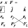
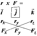
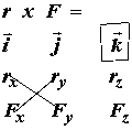
where F is the total force, Fx is the x component of the force, i is the unit vector along the x axis, Fy is the y component of the force, j is the unit vector along the y axis, Fz is the z component of the force, and k is the unit vector along the z axis.
Moments are defined as the vector cross product between the force vector and the vector between the point which the moment is about the the application of a given force vector:
![]() eq. 2
eq. 2
where x denotes the vector cross product defined as:
![]()
for the ith component of the resulting vector
![]()
for the jth component of the resulting vector
![]()
for the kth component of the resulting vector. The subscripts x,y, and z denote the x,y and z components of the corresponding vector, either the position vector r or the force vector F. Putting it all together, we have the following definition of the vector cross product in 3D for the moment calculation
![]() eq. 3
eq. 3
III. Static Equilibrium Equations (Statically Determinant Systems)
A body is said to be in static equilibrium if the sum if all the forces acting on the body are balanced and all the moments acting on the body are balanced separate from the forces. Balance of forces is termed translational equilibrium since forces will translate the body, while balance of moments is termed rotational equilbrium since moments will rotate the body. The best way to state the required balance of forces and moments is to break down the force balance equations into their x,y and z components. The resulting equations are:
 eq. 4
eq. 4where Fx are the x components of all the forces acting on the body, Fy are the y components of all the forces acting on the body, and Fz are the z components of all the forces acting on the body. We may write the same type of equations for the balance of moments:
 eq. 5
eq. 5As an example of static equilibrium calculation of muscle forces, consider calculating the force required to maintain upper limb position, example 2 in Chapter 1 of the text, as shown below:
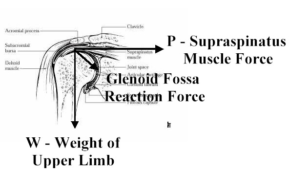
Based on the fact that the position vector r for all forces is zero, there are no moments for the three forces. Thus, the equilibrium equations reduce to translational equilibrium where the sum of the x component of the forces and the y component of the forces is zero. If we assume the angle between the glenoid fossa reaction force and the supraspinatus muscle force is 35 degrees, then we have the following equations:
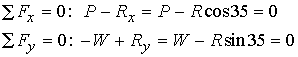
Given that the weight of the upper limb is 50 N, we can calculate the glenoid fossa humerus reaction force as R = W/sin35 = 87.1N. If we plug this result back into the balance of force equation for Fx, we obtain the muscle force necessary to hold the upper limb as 87.1N(cos35) = 71.3N.
The above example did not include moment balance for rotational equilibrium. Consider the following example (Example 3 in Chap. 1 in the text) with the forearm holding a weight (drawn only schematically):
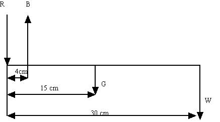
where R is the reaction force at the elbow, B is the muscle force for the biceps, G is the weight of the forearm and W is the weight in the hand. Let W = 20N and G = 15N. In this case, there are no force components in the x direction so we write only force balance in the y direction and a moment balance equation about the elbow. The force balance equation we can write directly as:
![]() eq. 6
eq. 6
For the moment balance about the z axis (coming out of the page), we need to calculate the cross product of the moment arm and the force vector for each applied force. The moment for the reaction force is zero since the moment arm is zero. For the biceps muscle we have the following force vector:
![]()
where the i and k components of the force are zero since the biceps force has only a j component. The moment arm vector is:
![]()
The j and k components are zero since the moment arm is 4 cm only in the x direction. Taking the cross product to obtain the moment we have:
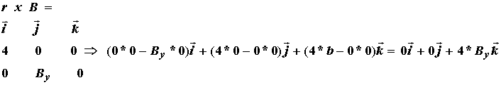
The cross product indicates that we only have a moment in the kth component or z direction. If we follow the same procedure for the other moments, which also only have z components, we obtain the following balance of moments:
![]() eq. 7
eq. 7
Assuming the forearm weight is 15N and the weight in the hand is 20N, we can solve directly for the biceps muscle force magnitude using the moment balance equation (eq. 7):
![]()
Please note that there is a discrepancy in the example in the text. The biceps moment arm is shown as 4cm in Fig.11, but taken to be 3cm in the text and equations. I have used 4cm in my calculations. We can now plug By into the force balance equation (eq.6) to obtain the reaction force as:
![]()
This example illustrates an important concept in biomechanics. Because muscles have short moment arms, they generally must generate large forces to balance external loads.
IV. Static Equilibrium Equations (Statically Indeterminant Problems)
In the above examples we were able to solve for unknown joint reaction and muscle forces using only the static equilibrium equations. However, in most cases of estimating muscle loads, we have redundant muscle forces. This means that there will be more unknowns than equations. Such systems are called statically indeterminate systems. Such a system is illustrated below (this is the example from Fig. 13, page. 17 in the textbook "Basic Orthopaedic Biomechanics"):

where the muscles left to right, their orientation and moment arms are as follows: 1. Biceps brachii (80.3 degrees from horizontal, 4.6 cm from elbow), 2. Brachialis (68.7 degrees from horizontal, 3.4 cm from the elbow) and 3. Brachioradialis (23 degrees from the horizontal, 7.5 cm from the elbow). Let us label the biceps force as Fbic, the brachialis force as Fbra, and the brachioradialis force as Fbrd. Let us assume that these muscles are acting to hold the forearm weight and weight in the hand for the problem we looked at previously. The simplfied Free Body Diagram is as follows:
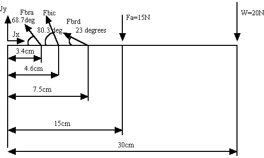
Based on the above free body diagram, we can directly write the balance of force equations for the x and y force components as:
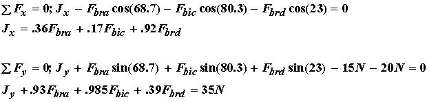
Next, we write the moment balance equation about the z axis. Since the x components of the force do not contribute to the moment (the moment arm is zero), we only have moments generated from the y component of the force. Using the stated moment arms, the moment balance equation is:
What makes this system indeterminate is the fact that we have 5 unknowns (Jx,Jy,Fbra,Fbic,Fbrd) and only 3 equations. This is a statically indeterminate system. This means that there are many possible combinations of values for the muscle forces that will satisfy the equilibrium equation. However, unless we find an alternate approach to solving for muscle force, we cannot find a unique solution.
In biomechanics, there are two widely used approaches to determining a unique solution: 1) Reduction methods and 2) Optimization methods. Reduction methods seek to reduce the number of unknowns to equal the number of equations. Reduction is accomplished using empirical reasoning, experimental data or a combination of the two. For instance, if two muscle groups have similar attachments and perform similar tasks, we may lump their force producing effort together into one muscle group, thus reducing the number of unknown muscle forces by 1. Or we use electromyography (EMG) to measure muscle activation signals, we may be able to deduce that a given muscle is not really active during an activity, again reducing the number of unknowns. The attractiveness of reduction methods is that we can use the same techniques to solve the muscle force problem and that the solution requirements remain relatively simple. This disadvantage is that we may make wrong assumptions, EMG data is often hard to correctly interpret, and we lose detail in terms of muscle prediction.
Reduction Approach Example
As a simple example for the reduction approach, consider the indeterminate system we consider with the forearm holding a weight. Indeterminancy arises because we have 5 unknowns and only three equations. In the reduction method, we would use information that would allow us to eliminate for example two of the three unknown muscle forces. For the first case, let us assume that the brachialis and the brachioradialis muscles are not active. Then we have three unknowns (the two components of the joint reaction force and the biceps muscle) and three equations. We can then use the balance of moment equation to solve for the biceps muscle force as:
![]()
The we can use the balance of force in the x direction and y direction to solve for the x and y components of the joint reaction force:
Jx = .17bic = 32.2N ; Jy = .985bic = 186.8N
Likewise, we could assume that the biceps and the brachialis muscles are not active and that only the brachioradialis muscle carries load. We again use the balance of moment equation to solve for the brachioradialis muscle:
![]()
We can then again use the balance of force in the x and y direction to solve for the x and y components of the joint reaction force:
Jx = .92brd = 259N ; Jy = .39brd = 109.8N
Note that depending on what muscles we assume are acitve, we obtain a very different solution even for the joint reaction force. This example shows how sensitive muscle force and joint reaction calculations are to assumptions about muscle activity in the reduction method.
In the second approach, optimization methods, we assume that muscles act together and are recruited in a manner that seeks to mimimize some objective. This has appeal from an evolutionary standpoint in that stronger species survive by using energy efficiently. Optimization techniques in general require numerical solutions. However, over the years they have been shown to be quite powerful in predicting muscle force distributions and are widely used to this day. We next discuss optimization methods and their application to estimating skeletal muscle forces.
Calculating Static Muscle Forces Using Optimization
I. Overview
We have seen that in most cases straight force balance equilibrium equations typically yield more unknown muscle forces than equations. This situation leads to an indeterminate problem or underdetermined problem. In this case, there are actually more than one solution that will satisfy the problem. We need to generate methods that allow us to make the problem determinate. In other words, we seek to alter the original problem so that we can find a solution. There are two general approaches to making a solution feasible. One is to reduce the number of unknowns using physical insights into the problem, such as experimental data. For instance, we may have electromyographic (EMG) data that suggests a muscle is not active during a specific activity. We may then choose to eliminate that muscle force from the equilibrium equations to reduce the number of unknowns relative to the number of equations.
The second approach to solve indeterminate muscle forces are a class of optimization techniques. Using these techniques, we seek the best solution among the many possible solutions that minimize some objective functional subject to constraints. Although there are many feasible solutions to an indeterminate muscle force problem, we seek the one that is "best" in some sense. For example, it may be the solution that minimizes the total stress in the muscle. This section gives a general overview of optimization problem statements and stationary conditions, followed by specific applications to determine muscle forces.
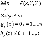
II. Mathematical Statement of Optimization Problem
The general formal statement of an optimization problem is shown below:
where F is a functional that depends on the variable x, a function Y that may depend on x, and the derivative of Y with respect to x. X is the variable with respect to which we minimize (or maximize) the functional F. In many optimization problems, especially those concerned with calculating indeterminate muscle forces, we may place restrictions on what values x may take as a minimizer. For instance, as we will see later on, we may want to minimize the total stress in a muscle, with a restriction that the muscles that are active must still produce a required moment about a joint. These restrictions are denoted as constraints. If we require that some function of x be equal to zero, that is an equality constraint. If we require that a function be less than or equal to zero or greater than or equal to zero, that is an inequality constraint.
When solving an optimization problem, it is helpful to know something about the nature of the problem since that will determine what numerical methods we may use to solve the problem. If only a functional F is to be minimized with no constraints, then the problem is an unconstrained miminization problem. If the functional F is linear with linear constraints, then that problem is generally termed a linear programming problem. If the functional F is quadratic with linear constraints, then the problem is termed a quadratic programming problem. If the functional F is nonlinear with nonlinear constraints, then the problem is considered a general nonlinear programming problem. For each of these general class of problems, there are specific numerical methods that may be applied.
III. Stationarity or Optimality Conditions Governing Optimization Problems
Although we generally cannot solve optimization problems analytically, we can derive conditions that the optimal solution must satisfy. These are known as optimality conditions, or also as Euler equations. The optimality conditions governing stationarity or optimality of a fucntional are analogous to the conditions characterizing the minimum value of a function. When determining the minimum value of a function, we take the derivative of that function and set that derivative equal to zero. This process yields an equation that when solved will give us the value of the variable that minimizers a given function.
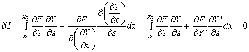
To find the governing equations of a function that minimizes a functional, we must turn to variational calculus, a branch of calculus that deals with functionals. To begin, consider that we wish to minimize a functional I that depends on x, Y (a function of x), and Y' (the derivative of the function of x). This functional is generically defined as:
 eq. 1
eq. 1
where I is the functional, x is the dependent variable, Y is a function of x, and e is a
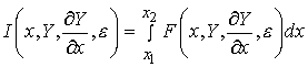
perturbation. We also impose boundary conditions on the functional such that Y(x1) = y1 and
Y(x2) = x2. We know that there is a function y that minimizes the functional I. However, there are many comparison functions Y that satisfy the boundary requirements but do not minimize the functional. We can denote the comparison functions as:
Y(x) = y(x) + eh(x) eq. 2
where h(x) represents a the addition to the function y(x). The functional I could represent for example an optimization problem to determine the minimum distance between points. This is illustrated below:
In the graph above, we see that in order for both Y(x) and y(x) to satisfy the end conditions, h(x) must be zero at x1 and x2, h(x1) = h(x2) = 0.
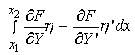
We next seek to minimize or extremize the functional I. In variational calculus, we take the first variation of the functional, denoted as dI, and set this to zero. With the comparison functions, we know that the minimum must occur with respect to e. Taking the derivative of the functions within the functional with respect to e we obtain:
 eq. 3
eq. 3
where we have applied the chain rule to differentiate F with respect to both Y and its first derivative with respect to x, which we denote Y'. We also note the following relations between the comparison function Y and the minimizing function y:
Y = y + eh
Y' = y' + eh'
we further note the following:
![]() eq. 4
eq. 4
using the results of eq. 4 in eq. 3 we obtain:
 eq. 5
eq. 5
We can integrate the second term in eq. 5 by parts to obtain:
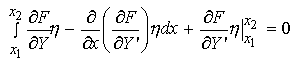 eq. 6
eq. 6
However, in our original characterization of h, h(x1) and h(x2) where required to be zero. Thus, we have:
 eq. 7
eq. 7
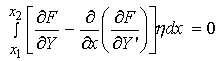
If F is continous, then for all smooth differentiable functions h with the added conditions that h vanish at the boundary, we can rewrite eq. 7, the variation of a functional as:
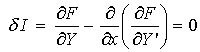 eq. 8
eq. 8
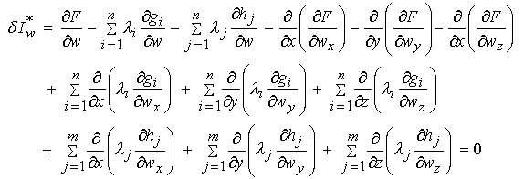
Equation 8 gives us the formula for calculating the first variation of a functional. Eq. 8 is also known as Euler's equation or the optimality conditions. In general eq. 8 generates a non-linear differential equation to determine the function that minimizes the functional I. The results of equation 8 are generally not used to solve for the minimizing functional. Rather, they are used to derive an iterative scheme to calculate the minimizing functional or used to check the results produced from other numerical optimization techniques. The variation of a functional is readily extended to three dimensional functions as:
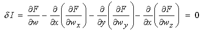 eq. 9
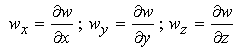
eq. 9Where now w denotes the design function within the functional I. Also, wx, wy, and wz are partial derivatives of the function w with respect to x, y and z respectively:
IV. Optimization Problems with Constraints
We derived the definition for the first variation of a functional (eq. 9), but did not consider that the function which minimizes a functional may be subject to various constraints given in the original mathematical statement for an optimization problem. To consider constraints in an optimization problem, we use the technique of lagrange multipliers. W
Using lagrange multipliers, we extend the original functional I to create an augmented functional I* that includes the constraints multiplied by lagrange multipliers. Suppose we return to our original definition of the mathematical statement of the optimization problem:
The original functional for this optimization problem would be:
I = F
To include the constraints, we would apply lagrange multipliers and create an augmented functional I*:
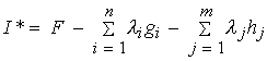 eq. 11
To find the function that minimizes the augmented functional I*, we take the variation of the functional with respect to all unknowns, including those associated with the constraints:
Now, in addition, we must take the variation of the augmented functional with respect to the lagrange multipliers. First, we take the variation with respect to the lagrange multipliers associated with the equality constraints g, which gives us i equations of the form:
![]() eq. 13
eq. 13
Next, we take the variation of the augmented functional with respect to the lagrange multipliers associated with the inequality constraints, which gives us j equations of the form:
![]() eq. 14
eq. 14
Note that the variation of the functional with respect to the lagrange multipliers gives us back the original constraints. In addition, we specify the additional condition that if the constrain is active, in other words, if the funciton is at the border or violating the constraint, the lagrange multiplier is non-zero. If the constrain is not active, then the lagrange multiplier is zero. These conditions along with the original constrains are known as the Karush-Kuhn-Tucker (KKT) conditions.
We now have all the necessary conditions to theoretically determine the minimizing function that satisfies the constraints.
V. Numerical Approaches to Solving Optimization Problems
The stationarity conditions derived above give conditions that any function that minimizes the given objective functional must satisfy. However, the equations are generally nonlinear and cannot be solved analytically. These equations are used to create a numerical approach to solve the optimization problem. These approaches are called optimality criteria approaches. They are more often used in structural optimization problems. In biomechanics, people generally use another broad approach to solve optimization problems termed mathematical programming approaches. There are a number of mathematical programming algorithms for solving optimization problems. However, the algorithms are geared towards specific types of probems and we most know how to classify these types of problems. In this section we review the different types of optimization problems and show how these problems may be solved using the Optimization toolkit in MATLAB. In the next section, we give an example of each problem and show how they may be solved.
1. Optimization Problem with Linear Objective Functional and Linear Constraints
One type of optimization problem we encounter in biomechanics is that of a linear objective functional with linear constraints, as shown below:
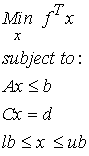
where x is the mimizing function, f is a vector of constants in the objective function, A and b are a matrix and vector respectively of inequality constraints, C and d are a matrix and vector respectively of equality constraints, and lb and ub represent lower and upper bounds respectively on the minimizing function x. Note that the linear programming problem follows the general mathematical description of the optimization problem.
Example:
As an example of a linear programming problem, let's consider the example 5 from the text, p. 19. The problem is stated below:
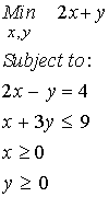
note that this contains the consitutents of a linear programming problem including a linear objective function, linear constraints and a lower bound on the minimizing functions. Also note that if we have no constraints, the answer will be the largest negative number possible for x and y, something that in a biomechanics problem is not physically feasible. This is often the role of constraints, making sure that the solution is physically feasible. Before presenting numerical approaches to the above problem, we illustrate the answer graphically, as in the text on page 20, Fig. 14:
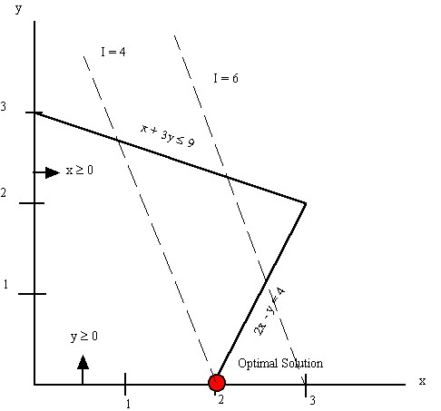
here I denotes the value of the functional and the optimal solution exists at x = 2 and y = 0. Note that this solution satisfies all the constraints of x and y greater than or equal to zero, 2x - y = 4, and x + 3y less than or equal to 9.
Now we show how this problem may be solved numerically, first in MATLAB, using the optimization toolkit. The appropriate function to use in MATLAB is linprog. In the example below, all MATLAB entries that you type I have put in bold. The >> symbol is the MATLAB command prompt. My comments about the commands are in red.
» diary -> This is the command to have MATLAB save all your command entries
» f=[2;1]; -> This is the input of the linear objective function, in our case 2x + y. In the MATLAB linprog you enter this as a vector. The vector is in brackets and each entry is separated by a semicolon. Also note that a semicolon after the command will prevent MATLAB from writing the command results immediately back to you. This corresponds to the minimization statement Min 2x + y.
» A=[1 3]; -> This is the input of the matrix coefficients for the inequality constraint matrix. Note that this is actually a two element vector and there are no semicolons between the entries.
» b=[9]; -> This is the right hand side of the vector for the inequality constraint. The A above and this vector correspond to the inequality constraint ![]()
» Aeq=[2 -1]; -> This is the coefficient matrix for the equality constraint. It has the same form as the equality constraint in our optimization problem 2x - y = 4. The Aeq gives the coefficients 2 and -1.
» beq=[4]; -> This is the right hand side vector of our equality constraint, the single number 4. This is again from 2x - y = 4.
» lb=zeros(2,1); -> This represents the lower bound on our minimization variables being ![]()
» [x,fval,exitflag,output,lamda]=linprog(f,A,b,Aeq,beq,lb);
-> This is the MATLAB toolbox command that is used to solve the linear programming problem. It is appropriately enough named linprog. All the matrix and vector entries we used in the defintion of the linear optimization problem are passed to the linprog solver as arguments. On the left hand side are the arguments that MATLAB will output when the iteration is terminated, either successfully or unsuccessfully. x is the solution vector, fval is the value of the objective functional at solution or last iteration, exitflag is a flag that tells you if MATLAB was successful in solving the problem, output is a structure variable giving full details of the optimization solution, and lamda are values of the lagrange multipliers.
Optimization terminated successfully.
» x
x = 2.0000 0.0000 -> after we input the linprog command with the required arguments, MATLAB gives us a message indicating that the optimization procedure was terminated successfully. We next type x at the MATLAB prompt (without semicolon so MATLAB will give a response) and MATLAB gives the components of the solution vector, 2 and 0. Note that these (as we would hope!) match the solutions we obtained from the graphical solution.
» fval
fval = 4.0000
» exitflag
exitflag = 1
2. Optimization Problem with Quadratic Objective Function and Linear Constraints
A second optimization problem encountered in biomechanics is that of a quadratic objective function with the same linear constraints as the linear programming problem. This problem is defined below:
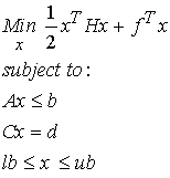
The above problem is known as a quadratic programming problem, where x is the minimizing function, H and f are a matrix and vector of constants respectively in the objective function, A and b are a matrix and vector respectively of inequality constraints, C and d are a matrix and vector respectively of equality constraints, and lb and ub represent lower and upper bounds respectively on the minimizing function x. Let's consider another example solving a quadratic programming problem in MATLAB. For this case, we consider the example problem in the MATLAB manual. This is stated as follows:
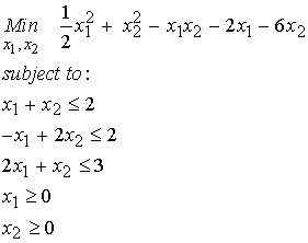
Note that the highest order terms is squared and that all the constraints are linear functions of x1 and x2.
In MATLAB the generic quadratic programming problem is defined as:
The quadratic programming solver is again appropriately labeled quadprog in MATLAB. To utilize this solver, we must enter the matrices H, A, Aeq, and the vectors f, b, beq, lb, and ub for the MATLAB quadratic programming defintion. The MATLAB session is thus:
» H = [1 -1; -1 2] -> H is the matrix of the quadratic part of the objective function. This is a 2x2 matrix
» f = [-2; -6] -> This vector is the right hand side of the inequality constraint
» A = [1 1; -1 2; 2 1] -> This matrix is the left hand side coefficients of the inequality constraint
» b = [2;2;3] -> This is the right hand side of the inquality constraint matrix
» lb=zeros(2,1) -> This is the lower bound constraint on x1 and x2.
» [x,fval,exitflag,output,lambda]=quadprog(H,f,A,b,[],[],lb)
-> This is the solution of the quadratic programming example. The output are the same as for the linear programming example: x is the solution vector, fval is the value of the function at the solution, exitflag telling whether the optimization solution is successful. Lamda is the lagrange multiplier for the solution. On the right hand we enter the matrices H, A and the vectors f,b, and lb. Since there are no equality constraints, we leave Aeq and feq blank.
x = 0.6667 1.3333 -> The solution vector is x1 = .6667 and x2 = 1.333.
fval = -8.2222 -> The function value at solution is -8.2222.
3. General Nonlinear Optimization Problem - Nonlinear Programming
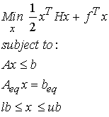
If an optimization problem is defined with a nonlinear objective function of a degree greater than 2 (even with linear constraints) or has nonlinear constraints, then the problem is termed a general nonlinear optimization problem or nonlinear programming problem. The general mathematical form of the nonlinear optimization problem is given below:
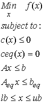
where f(x) is a general nonlinear objective functional, c(x) is a general nonlinear inequality constraint, ceq(x) is a general nonlinear equality constraint, Ax is a linear inequality constraint, Aeqx is a linear equality constraint, and lb and ub represent lower and upper bounds on x, respectively.
To solve the general nonlinear programming problem in MATLAB, we utilize the command fmincon. However, in contrast to the other solution techniques we've consider, for fmincon we need to write a function defined in a ".m" file to evaluate the nonlinear objective function and any general nonlinear equality or inequality constraints. This is because these functions may have any form unlike the linear or quadratic functions.
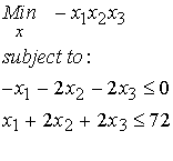
We next consider a the general nonlinear optimization problem used as an example in the MATLAB Optimization toolbox manual:
The following are the MATLAB commands to solve the nonlinear optimization problem above. First, we define the .m file containing the function evaluation:
function f = optfun(x) -> This is the .m file defining the objective function
f = -x(1)*x(2)*x(3)
This is saved in a file called optfun.m. Next since all the constraints are linear, we may use the form Ax is less than b. These are input as:
» A=[-1 -2 -2;1 2 2] -> This is the coefficient matrix for the linear equality constraint
» b=[0;72] -> The is the right hand side for the general linear inequality constraint
The next thing we need is a guess for the initial values of the function. As in the manual, we enter:
» x0 = [10;10;10]; -> This is the initial guess for the optimization solver
We then run the general nonlinear program solver as:
[x,fval]=fmincon('optfun',x0,A,b) -> This is the calling of the general MATLAB command for nonlinear programming. x is the solution on ouput, fval is the value of the function at output. 'optfun' is the name of the file that evaluates the objective function. x0 is the vector containing the initial starting point, A and b are the coefficient matrix and vector for the linear inequality constraint.
On return, MATLAB gives x1 = 24, x2 = 12, and x3 = 12. The function evaluates at solution to -3,456.0
VI Optimization Approaches for Estimating Muscle Loads
The idea of utilizing optimization approaches to estimate muscle loads has permeated biomechanics research for the last 30 years. Even before this time, the idea that the body moves in an efficient or optimal manner has been popular. The Weber brothers in 1836 proposed that humans walk in a manner that costs the lightest energy expenditure for the longest time and gives the best results. A popular optimization criteria is that the sum of the muscle forces is minimized. This is a linear programming problem, and generally gives the result that only one muscle force is active at a time. This is contrary to experimental results that show generally more than one muscle active across a joint.
One significant improvement in optimization criteria was proposed by Crowninshield and Brand in 1981 ("A Physiologically Based Criterion of Muscle Force Prediction in Locomotion", J. Biomechanics, 14:793-801). This paper tried to take physiological considerations into account when formulating the optimization problem. They based their idea of optimization based on the idea that muscle fatigue is related to the physiologic stress in the muscle, defined as the force divided by the physiologic cross-sectional area of the muscle. It is widely known that muscles can sustain high amounts of force for short periods of time and lower forces for longer amounts of time. In fact, the amount of time that a muscle can sustain activity is inversely proportional to the muscle stress raised to the third power.
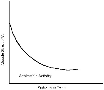
Based on the graph above, Crowinshield and Brand proposed that the optimization criteria of the body was to minimize muscle stress raised to a power, with the constraint that the muscles need to generate the required moment about a joint that is necessary to perform a task. In other words, they proposed that the body recruits muscles in a manner as show to minimize fatigue. Mathematically, this optimization criteria may be written as:
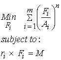
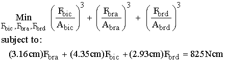
where Fi are the individual muscle forces, Ai is the individual muscle cross-sectional area, n is a user chosen exponent, ri is the moment arm vector of each muscle and M is the total moment about the joint. Note that the moment constraint is linear. Depending on the value of n, the Crowninshield and Brand criteria may yield a linear programming problem (n=1), a quadratic programming problem (n=2) or a general nonlinear programming problem (n>2). Let's consider the above optimization formulation applied to the indeterminate problem of holding a weight in your hand. The muscle forces are again the biceps Fbic, the brachialis Fbra, and the brachioradialis Fbrd. Lets denote the corresponding physiologic cross-sectional areas of these muscles as the biceps area Abic, the brachialis area Abra, and the brachioradialis area Abrd. We can then write the objective function for the Crowninshield and Brand approach to this problem as:

The constraint on this approach is that the total moment generated by the muscle forces about a joint must balance the total externally applied moment about the joint. In this case, the total externally applied moment is the weight in the hand and its moment arm plus the forearm weight and its moment arm. This we calculate as:
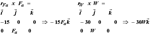
We then obtain the total external moment as 15cm*15N + 30cm*20N = 825Ncm. Utilizing the moment balance equation we originally calculated under static equilibrium for this problem, we obtain the moment constraint as:
![]()
Thus, the complete optimization problem statement for the Crowinshield and Brand approach for the indeterminate forearm problem can thus be written as:

Next, we solve the above equation using different values of n for the exponent and compare the results. If we assume n = 1, we have the following optimization problem:
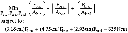
The above problem can be classified as a linear programming problem, since both the objective function and the constraints are linear functions of the minimizing variables Fbic, Fbra, Fbrd. To utilize MATLAB for solving the linear programming problem, we need to use the MATLAB form of the linprog solver. Thus, we rewrite the above as:

We obtain the muscle physiologic cross sectional area from An et al. (An, K.N., Kwak, B.M., Chao, E.Y., and Morrey, B.F., "Determination of Muscle and Joint Forces: A New Technique to Solve the Indeterminate Problem", J. Biomechanical Engineering., 106:364-367, 1984): Abic = 4.6sq.cm, Abra = 7.0sq. cm, Abrd = 1.5sq. cm. We are now ready to solve the optimization problem using MATLAB:
» f=[1/4.6; 1/7.; 1/1.5] -> Input coefficients for objective function, in this case 1/Area of muscle
» Aeq=[4.35 3.16 2.93] -> Input matrix coefficients for equality constraint, in this case the moment arm
» beq=[825] -> Input right hand side of constraint
» lb=zeros(3,1); -> Since we know by the mechanics of the problem that the moments have to be positive, we impose a lower bound constraint; Otherwise, MATLAB does not reach a solution.
» [x,fval,exitflag,output,lamda]=linprog(f,[],[],Aeq,beq,lb); -> Run the MATLAB solution using linprog. Note that since we don't have inequality constraints, we use empty brackets for the matrix left hand side and vector right hand sides where the inequality constraint matrix would normally be.
» x -> we type x to get the solution vector
x = 0.0000 261.0759 0.0000 -> we see that the optimization solution predicts that only the bracialis muscle will be active and that it will generate 261 N of force to lift a weight of 20N.
» fval fval = 37.3078 -> this tells us that the value of the objective function at the minimum is 37.3
It is interesting to note that if we apriori assume the both the biceps muscle force and the brachioradialis muscle force are not active, we obtain the same answer by static equilibrium:
![]()
Next, let's use n = 2 as the exponent in the optimization problem. We know have the problem defined as:
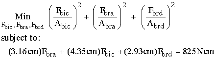
To again put this in a form of the quadratic programming problem that MATLAB recognizes, we write:
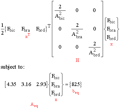
For the quadratic programming problem Aeq and beq are entered as they were for the linear programming problem. We run the following MATLAB session to solve the optimization problem when n = 2:
» H = [2../4.6^2 0 0; 0 2../7^2 0; 0 0 2./1.5^2] -> This is the matrix of coefficients for the quadratic part of the quadratic programming problem. Note that in this case there is no linear component.
» f=[0 0 0] -> We enter the matrix f as zeros since there is no linear portion to the objective function
» [x,fval,exitflag]=quadprog(H,f,[],[],Aeq,beq) -> Here we run the MATLAB solver. Note again we use empty brackets because there are no inequality constraints. In this case we also do not use a lower bound on the muscle forces.
x = 83.5391 140.5297 5.9832 -:> when we type x we get the solution vectors.
We see that as we increase the exponent to 2, more muscles are predicted to be active. The biceps now generates 83 N of force and the brachioradialis now generates 4.8N of force. The force in the brachialis muscle now actually is reduced to 142 N.
Finally, let's consider the case where n > 2. If we take n = 3, the optimization problem may be stated as:
This problem now corresponds to the general nonlinear programming problem because the objective function has a different nonlinearity than a squared or quadratic function. To solve this problem, we use the fmincon solver in MATLAB. Recall that when using fmincon, we must write a function to input the objective function and any nonlinear constraints. The .m file we write contains the following statements:
function f = crownnonlin(x)
f = (1/4.6^3)*x(1)^3 + (1/7.^3)*x(2)^3 + (1./1.5^3)*x(3)^3
We then input the equality constraint coefficient matrix and right hand side vector as in the linear and quadratic programming solutions. Finally, in the case of the nonlinear programming problem, we enter an initial starting guess for the solution.
» x0=[0; 0; 0]; -> Enter 0,0,0 as the initial guess
[x,fval,exitflag]=fmincon('crownnonlin',x0,[],[],Aeq,beq); -> run fmincon to solve the general nonlinear programming problem. Use the function defined in crownnonlin.m to evaluate the objective function.
We obtain the following solution:
» x
x = 95.7179 69.5330 64.4720
Thus we see even a more evenly distributed force distribution between the three muscles. In this case, the biceps muscle generates the largest force at 95.7N, then the brachialis at 69.5N and the brachoradialis at 64.5N.
As Crowninshield and Brand discuss in their paper, as the exponent in the objective function increases, the force generation is more distributed among the muscles to reduce the onset of muscle fatigue. Experimental validation of their approach analyzing muscle force generation compared to EMG of muscle activity shows some correlation.
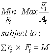
Another optimization approach proposed to predict muscle forces is that of An et al. that we referenced earlier for data on muscle cross-sectional areas. They proposed a linear programming method with additional constraints to address the concern that most linear programming methods predict that only a few muscles will be active during an activity. They also justified their method based on the fact that nonlinear programming methods can be very sensitive to ill-conditioned data and therefore convergence to a solution cannot be guaranteed. In their approach, they propose using the moment balance equation as a linear equality constraint just as Crowninshield and Brand. However, in addition, they also propose an linear inequality constraint on the maximum muscle stress, while at the same time minimizing the maximum muscle stress. We may formally state this problem as:
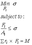
To solve this problem in MATLAB, we assume that the maximum value F/A will be equal to s. Then the problem can be rewritten as a minmax problem:
In MATLAB, we solve this type of problem using the fminimax solver. To use this solver, we again need to write a function in a .m file. This function is shown below:
function f = anfun(x)
f(1) = (1/4.6)*x(1)
f(2) = (1/7.)*x(2)
f(3) = (1./1.5)*x(3)
Notice that we have a set of functions f(1), f(2), and f(3) in addition to the minimizing vector x. We enter the linear equality constraints as before run the minimax solver as:
[x,fval,exitflag]=fminimax('anfun',x0,[],[],Aeq,beq); -> input initial guess, .m function to evaluate objective function, and equality constraints.
We obtain the following solution:
x = 81.5690 124.1268 26.5986
with a biceps force of 81 N, a brachialis force of 124 N, and a brachioradialis force of 26.6 N. If we look at the value of the set of functions we obtain:
fval = 17.7324 17.7324 17.7324
This indicates that the stress in each muscle is equal!
Below we summarize the results for our model statically indeterminate problem using the different formulations:
Formulation Biceps Brachialis Brachioradialis Moment
Crown/Brand n = 1 0N 261N 0N 825Ncm
Crown/Brand n = 2 83.5N 140.5N 6.0N 825Ncm
Crown/Brand n = 3 95.7N 69.5N 64.5N 825Ncm
An Min Max s 81.6N 124.1N 26.6N 825Ncm
If we calculate the stress in each muscle we obtain:
Formulation Biceps Brachialis Brachioradialis
Crown/Brand n = 1 0MPa .372MPa 0MPa
Crown/Brand n = 2 .18MPa .200MPa .040MPa
Crown/Brand n = 3 .21MPa .100MPa .430MPa
An Min Max s .178MPa .178MPa .178MPa
An important point to note is that different optimization formulations and assumptions lead to different predictions of muscle forces. Again, when applying the different optimization formulations, one should look at the underlying assumptions and how they relate to a physiologically established criteria like muscle fatigue or muscle stress. However, it is important to note that the muscle stress as noted in these formulations is gross muscle stress, ie it is an average stress over the whole muscle. This stress does not tell us what stresses individual sarcomeres or muscle cells see, which is important when we are looking at damage in the muscles. To understand this level of stress better, we need a hierarchical view of tissue structures and mechanics, which forms the basis for much of what we will do in the upcoming lectures.
VI Verifying Optimization Solutions
It is in general very difficult to completely verify optimization solutions experimentally. One method is to compare the results against experimental EMG data. This is a commonly used baseline. This verification goes to the basic assumption about how muscles are recruited and how muscle force is generated in a certain activity. Another verification question is whether our numerical solution scheme has achieved the best answer to the statically indeterminated problem. This again, is difficult to verify directly. A baseline check is to make sure that the solution obtained via the numerical optimization solution satisfies the equilibrium equations. Note that when the moment balance equation is used as a constraint we generally satisfy this equation.
The next level in validation is to use the optimality criteria equation from variational calculus. This equation holds for any optimization formulation with an objective function that has greater than linear force functions. Let us show how this can be applied to the Crowninshield and Brand approach with the exponent n = 2. The augmented Lagrangian can be formed as:
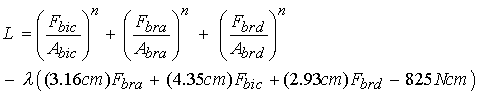
We next take the variation of the augmented Lagrangian with respect to each muscle force and the Lagrange multiplier l. This gives us the following:
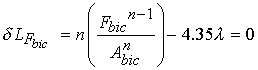
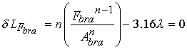
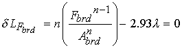
![]()
We next solve for the lagrange multiplier l using the variation of the augmented lagrangian with repsect to the biceps force (first of the four equations) to get:
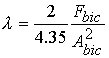
If we substitute for the lagrange multipliers into the equation for the brachialis force (bra) and the brachoradialis force (brd), we get the following relationships between the magnitude of the muscle forces:
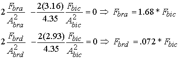
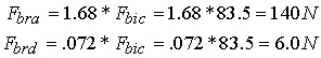
Using the values for Fbra, Fbic,and Fbrd from the results table comparing approaches, we obtain:
The optimality criteria equations provide us with a method to check the validity of the numerical solution. Thus, to summarize, we may check the validity of the numerical solution by the following steps:
1. Check to see if the optimization solution satisfies equilibrium equations
2. Check to see if the optimization solution (for other than linear programming problems) satisfy the optimality criteria equations.
To determine if the optimization formulation is valid experimentally, we must check the predicted muscle forces against some experimental measure, in most cases EMG data.