 for frequency, and
  for wavelength. The symbol `c' is used for the velocity of
light, thus:
for wavelength. The symbol `c' is used for the velocity of
light, thus:
Until the development of the space program, virtually all of the astronomers' information came in the form of light from distant objects. It is natural that they would have played an important role in the investigations of the nature of light, just as they did in the development of Newton's mechanics. Many of the pioneers in the development of the modern theory of light were keenly interested in astronomical problems.
The true nature of light wasn't really understood until the 20th century. Experiments done in the 19th century indicated that light was a form of wave motion. For many purposes, it is sufficient to describe light as a combined electrical and magnetic wave, or an electromagnetic wave.
In the decade following 1964, the great English physicist James Clerk Maxwell was able to describe all electrical and magnetic phenomena with the help of four differential equations. They are now called Maxwell's equations, and every student of physics must learn to work with them.
It's quite amazing that phenomena as varied as starlight, and children's magnets could be described by four relatively short equations, but this is the case.
Perhaps the simplest way to think of these waves is to first picture ``lines of force'' about an electrical charge. Nearly everyone has seen the lines of force about the poles of a magnet demonstrated with the help of iron filings and a glass plate. The concept of lines of force arose as a way of eliminating the problem that arose with the attraction of two bodies separated by some distance.
It's easy enough to understand how something will move if you grab it and push or pull. On the other hand, how can two bodies separated by "nothing" attract or repel one another? This difficulty is known as the problem of action at a distance. It can be solved, after a fashion, with the notion of lines of force. Think of electrical charges or magnetic poles as being surrounded by lines of force, like those demonstrated for a bar magnetic. Then the lines of force fill in the void between the bodies. They will grab the other body, and there is no more action at a distance.
Maxwell's equations described these lines of electrical or magnetic force. They showed that if you accelerated a charge, for example, if you wiggled it up and down, a wave would run out the electrical line of force.
The same equations showed that the electrical wave would have to be accompanied by a magnetic wave. That's a little hard to see, and we won't go into it here. Take our word for it. But the electrical wave can be pictured as something similar to the wave that would travel down a rope. Stretch a rope out horizontally, and wiggle one end of it, and a wave will run down the rope away from your hand. Pretend that you fasten the far end way away, so you don't have to worry about what happens when the wave gets to that end.
The electromagnetic wave is a form of light. It turns out that light is most conveniently described as a wave when the wavelength is relatively long, say of the order of a centimeter or more. Radio waves can be tens or even hundreds of meters in wavelength.
All wave motion travels with a velocity equal to it's frequency
(units are per second, or sec-1) multiplied by its
wavelength. Astronomers traditionally use the Greek letter
for frequency, and
for wavelength. The symbol `c' is used for the velocity of
light, thus:
= c
When the wavelength of light is shorter, a millimeter or less, say, a rather different picture is better--the photon picture.
According to the quantum theory, the energy in electromagnetic waves comes in little bundles that are called photons. The shorter the wavelength, the better it is to think of the photon as a kind of particle--rather than a wave. It isn't that the wave picture becomes invalid, it's just that for many purposes, it's better to think in terms of photons.
Light, X-rays,  -rays, and radio waves are thus all forms of the
same phenomena--electromagnetic radiation.
-rays, and radio waves are thus all forms of the
same phenomena--electromagnetic radiation.
In 1900, the German physicist Max Planck was trying to understand the nature of radiation that filled an enclosure that had come to equilibrium. When temperature within the enclosure was the same everywhere, people measured the amount of energy in the radiation as a function of wavelength. Their results could be displayed as a kind of histogram, with energy plotted against small wavelength intervals. What they found was quite surprising. The shapes of the curves depended only on the temperature of the enclosure, and not on the material inside. Planck himself made many of these measurements, and the energy distribution became known as the universal Planck radiation law.
The German word for this kind of a distribution of electromagnetic radiation literally means "radiation from a cavity." The equivalent English term is black body radiation. One can blacken a surface with paint, or better, with soot, and it will emit radiation that is (very nearly) in the form of Planck's universal law.
Planck found that he could account for this law with the help of
Maxwell theory provided he assumed that the energy in the radiation
came in multiples of the frequency: E = h.
The constant quantity `h' is now known as Planck's constant, and it is one
of the three fundamental constants of nature. The other two are the
constant of gravitation G, and the velocity of light, c.
The most energetic forms of electromagnetic radiation are called
-rays. These photons are characteristic of the emissions of
atomic nuclei, and have energies of millions of electron volts
(MeV). X-rays are slightly less energetic, with energies of
thousands of electron volts, kilo-electron volts, or KeV. The
photons of visible light have energies of the order of a few electron
volts (eV).
   Name              Energy           A Characteristic Wavelength
   ----              ------           ----------------------------
   Gamma rays          Mev                  0.01 Angstroms
   X-rays              KeV                 1    Angstrom
   visible light       0.2 eV                5000 Angstroms
   infrared light                            0.003 cm
   microwaves                                1 cm
   radio waves                              100 meter
There are other forms of "radiation" that are not electromagnetic.
The famous "rays" of radioactive material were called  ,
,
 ,
and . Of these, only
rays are electromagnetic. The
and rays are helium nuclei
and electrons, respectively.
,
and . Of these, only
rays are electromagnetic. The
and rays are helium nuclei
and electrons, respectively.
The first astronomical telescopes were made by Galileo. They used a lens and an eyepiece. Such telescopes are called refractors because the light is bent by these lenses. The bending of light is called refraction. Galileo's eyepieces allowed him to see the images right side up, just as binoculars do. It turns out to be a little more efficient if one can live with an upside down image. The traditional astronomical telescope inverts the image. This is not a disadvantage when viewing celestial objects, for which we may have no preconceived notion of how they should be oriented.
For many years, astronomers made upside down maps of the Moon, because that was the way the Moon appeared in their telescopes. Even in recent textbooks on astronomy, one can see photographs of the Moon that are upside down. Planetary astronomers prefer to have the north at the top of a map, however, and gradually most lunar maps have appeared in that orientation.
The largest refracting telescope is the 40" at the Yerkes Observatory of the University of Chicago. It, and the Lick 36" were built at the end of the 19th century. Early in the 20th century these instruments were surpassed by large reflecting telescopes. The 60" reflector Mount Wilson went into operation on Mount Wilson, California in 1908, followed by the 100" reflector in 1917. The latter was the world's largest telescope until the 200" reflector was completed at mid-century, and placed on Palomar Mountain. As our century ends, numerous larger telescopes have gone into operation. Currently the largest are the twin Keck telescopes in Hawaii, which have the light-gathering equivalent of 10 meter telescopes.
Telescopes have 3 roles or functions
is the ratio
/D, where D
is the diameter of the primary. This ratio comes out in radians, and is
often converted to seconds of arc. There are 206265 seconds of arc in a
radian. Higher resolving power traditionally means the ability to
see objects separated by a smaller angle.
Telescopes may be characterized by 2 numbers, the diameter of the primary (mirror or lens) and the focal length of the primary. The focal length is the distance from the primary at which an image is formed by light rays coming from infinity.
All of the newer major telescopes are reflectors, because it is possible to make them bigger than lenses. The current new telescopes are of the order of 8 meters in diameter. By putting many mirrors together, the effective aperture has been increased to 10 meters. Reflectors are free from chromatic aberration, which distorts images formed by lenses. If a telescope used a simple lens, the blue light would come to a focus before (closer to the lens) than the red.
Mirrors have distortions too. In particular, light rays near the axis of the mirror may not come to the same focus as rays near the edge. This effect is called spherical aberration. It was the problem that affected the Hubble Space telescope.
Our Earth's atmosphere is transparent to light only from about 3200 to 10,000 Angstrom units. One Angstrom is 10-8 cm. Shorter and longer wavelengths are blocked by various absorbers. At much longer wavelengths, there is an important radio window, from about a centimeter to perhaps 10 meters.
The atmosphere not only absorbs radiation at wavelengths astronomers would like to observe at, it also distorts images--the twinkle of stars results in a distortion. So space observations are important, and the Hubble Space Telescope has been making many important discoveries.
The outer rim of the Hubble primary is too low, giving rise to spherical aberration. After three years of sub-standard performance, a servicing mission installed corrective optics, and the instrument is now performing to expectations.
Photography came into its own in the latter half of the 19th century. All of the early astronomers before this time were visual observers. They had to record their observations in the form of sketches, and some of them got to be pretty fanciful. The Earth's atmosphere distorts the images of stars and planets, so in a very real sense, observers couldn't really see the same things.
The problem came to a head in the case of observations of Mars, where the American astronomer Percival Lowell claimed to see elaborate markings, which he interpreted as artifacts from an advanced civilization. Other astronomers saw nothing like the amount of detail in Lowell's sketches.
Photographic plates of Mars showed even less detail than visual observers could see. This is because the plates were essentially long exposures; the flickering images of the planet were blurred. Visual observers could wait for moments of exceptional "seeing," and it was at those times that Lowell claimed to see things no one else could.
For most of the 20th century, the traditional astronomical detectors were photographic plates. They were widely used in astronomy toward the end of the last century, continuing to well past the middle of the current one. Quite wide fields may be photographed, and this is still one of the major strengths of astronomical photography. However, only about 1 to 2% of the light falling on a photographic plate is detected. This drawback not present with modern electronic detectors; the most common is called the CCD, or charge coupled device.
CCD's were invented at Bell Labs in the mid 1970's. Unlike photographic plates, they detect 90% or more of the light that falls on them. However, they are still small in size, the largest ones being about 2 inches on a side. They are also expensive.
CCD's operate on the basis of the interaction of light photons and silicon crystals. Photons in a certain wavelength interval are capable of freeing electrons within the crystal so they can be made to move as in ordinary electrical current. The freed electrons are maintained in the original locations by electric fields generated as a part of the detector. These fields are said to generate potential wells, which we may conceptually think of as little bowls in which the electrons collect. The more electrons, the more light photons that hit the silicon. It is possible to localize these potential wells in to very small areas, so that the resolution of modern CCD's approaches that of photographic plates--10 to 20 microns (1 micron is 10-4cm).
After a time, the charge in the wells represents a digitized version of the image. It is then possible to manipulate the wells in such a way that the charge in each of them may be measured. In essence, the charge (or number of electrons) in each well is read one by one, in such a way that the location of the charges is remembered. The image may then be reconstructed by a computer. To do this by hand would take quite a while. A modern CCD might contain 20 Megabytes of data!
With a photographic plate, or with a CCD, the most elementary technique
is called imaging--just a fancy way to say "taking a picture."
Images of star fields were traditionally measured carefully for the
positions of stars, to reveal their proper motions or parallaxes.
The images of extended objects, such as bright or dark gas clouds, or of
external galaxies would simply be examined and their characteristics
noted. Photographic images of galaxies led Edwin Hubble to his famous
tuning-fork classification scheme.
Extensive imaging from space probes have been used to advance
our knowledge of the solar system. Even before the lunar missions,
planetary geologists had begun to map the surface of the Moon using
techniques that had been developed by terrestrial geologists.
We had to wait for space probes before the same methods could
be applied to the planets. Telescopic images of Mars,
both visual and photographic, had led
to more confusion than enlightenment. Mariner and Viking images
of Mars in the 1970's, revealed a surface intermediate in complexity
between those of the Earth and Moon.
A standard technique for the analysis of an extended source such
as a planetary surface is to make plots that indicate areas with
equal brightnesses. Astronomers call such plots isophotes,
and they resemble contour maps, except that brightness rather than
altitude are indicated. With digital information, it is possible
to display brightness with color rather than contours. Such
false color maps are now used in a wide variety of scientific
applications.
It was known to Isaac Newton that if sunlight was passed through a
polished glass prism, it would be dispersed into a rainbow of colors.
This is illustrated in Figure 13-2
During the 19th century, physicists learned how to use this technique
to identify chemical elements in a laboratory sample. At the same
time, similar methods were employed as a means to analyze the
atmospheres of the sun and the stars. If the dispersed light is
examined with the eye, the instrument is called a
spectroscope.
If that light is first recorded with a photographic plate, or
electronic detector, the term spectrograph is used.
The light itself, after dispersion, is called the spectrum
of the object that emitted it. The plural of spectrum is spectra.
It was already recognized that the nature of the spectrum
of an object depended on physical conditions.
Gustav Kirchhoff's
laws of
spectroscopy are
valid today:
It was soon realized that one could identify the chemical element
by its bright or dark spectral lines. There is a story that Kirchhoff
once told his banker that he had identified the chemical element gold
in the spectrum of the sun. The banker was unimpressed, because
there was no way to mine that gold. Later, Kirchhoff was awarded
a gold medal from the British Royal society, along with some gold
coins. He is said to have returned to his banker, saying "this is
gold from the sun."
Modern spectrographs generally employ gratings rather than prisms
as dispersing elements. Gratings can be used either in transmission
or reflection. In the latter case, a mirror is closely ruled with
parallel scratches. The light that bounces off such a surface is
dispersed into little rainbows on either side of a central image,
called orders.
It has become possible to make these scratches so that most of the
light is thrown into one of these orders. Such a grating is said
to be blazed, and can be a very efficient dispersing element.
Atoms, electrons, and nuclei no longer obey Newton's "classical" laws.
The modifications are not intuitive. You have to learn the rules, and
that takes some effort. For our purposes, we can examine the case of
a very
simple system, a hydrogen atom consisting of an electron and a proton.
The two relevant charges, are the same in this case, and
the attractive force is is an inverse square one, just as for
gravitation. The potential energy curve is proportional to 1/r,
and looks just like the one for the two-body problem [Figure 11-2(b)].
Quantum rules prevent the electron from being at any (old) distance
from the proton. If we drop the electron straight at the proton, then
there are a series of distances where the electron will "hang" on its
way down the well.
It is the wave nature of the electron that makes it "hang" at certain
depths in the potential well. It turns out that when you examine the
wave nature of the electron, its wave has just one loop at the
lowest possible energy level,
2 loops at the next one up, and so on. The picture is a
little more complicated if we add angular momentum, but we don't
need that here. There must be an
integral number of waves in the well or the corresponding energy
isn't allowed. This is why the energies
are said to be quantized.
On the way to higher energies, the allowed levels crowd closer and
closer together.
Electrons can get from one level to another by emitting or
absorbing a photon of just the right energy. This is an example
of the famous quantum jump. For a jump down, a photon
must be emitted, and for a jump up, one must be absorbed. These
photons are created when the electron jumps down, and are destroyed
when it jumps up. So the energy of the photon, h If a photon of frequency We can understand the Kirchhoff laws with the help of this quantum
picture. First [see K1 above], we get a continuum when the energy levels get
very close together. This can happen in solids (like a tungsten
filament) and liquids. When the atoms are very near one another, the energy
levels get smeared out and their average values can also get close together.
This will also happen to a gas under high pressure,
such as the visible photosphere of the sun.
When [K3] a continuous spectrum
shines through a cool, low pressure gas, the atoms in the gas selectively
absorb out the discrete wavelengths determined by their special
energy levels: E1, E2, E3, etc.
If a hot gas is observed without a continuous source behind it,
some fraction of the atoms in this gas will always be in higher energy
levels. They can get into these upper levels in a variety of ways.
They can bump into one another, and get boosted to higher internal
energy states. What happens in that some of the kinetic energy of
motion in transformed into internal energy. Also the hot gas
may absorb occasional photons from some other source. These
photons may boost the electrons to upper levels, or even ionize
the atoms. Eventually, the electrons will recombine and/or just
jump to lower energy levels, with the emission of a photon. When
these photons are observed, they show a bright-line, or emission
spectrum [K2].
Radio telescopes function much like optical ones. Their primaries
are often parabolic reflectors, but much larger. The same formula,
The large, often parabolic receivers that one sees in pictures of
radio telescopes function rather like the antennae of ordinary radios.
The electromagnetic waves from space are made to drive electrical
currents which
are then subject to ingeneius and powerful amplification. You can often
read about radio astronomers "listening" to sounds from space. The
signals received are electromagnetic, and not acoustical. The popular
notion of listening comes by analogy to "listening" to an ordinary
radio. The electrical currents can be made audible with the help
of speakers. Often, radio astronomers employ speakers, and do listen
to their sounds. Unlike the sounds from an ordinary radio, the
sounds from speakers at a radio telescope mostly resemble static.
Astronomers are keenly interested in signals from deep space that
are carried by high energy photons, X-rays and In
planetary astronomy, this region of the electromagnetic spectrum is
chiefly employed in the overall technique called remote sensing,
which we will discuss in detail later in the course.
Electromagnetic radiation comes in many forms. In order of increasing
wavelength, and decreasing energy and frequency, we have:
Light is analyzed with the help of spectrographs. Astronomers
have used both prisms and gratings to disperse light.
Each atom and ion has a set of unique energy levels. Transitions
or quantum jumps among these levels give rise to the emission or
absorption of photons. Kirchhoff's laws describe the conditions for
continuous, absorption, or emission spectra. Chemical elements
can be identified by measuring the wavelengths of light that
are emitted or absorbed by some source.
What does it mean to analyze cosmic materials? What information
would we have after such an analysis that we didn't have before?
There are a variety of ways cosmic materials may be analyzed.
The simplest kind of question we might ask is for the number
of atoms of each chemical element in the sample. So we can
think of the periodic table, and having a number for each element.
A chemist would think in terms of the number of "moles" rather
than numbers of atoms, but if we know Avogadro's number
(Na) we
can give the information either way.
If we take a sample and divide it into several parts, the
number of atoms in each part will be different, in general.
If the sample is uniform--not different in one place than
another--the relative numbers of atoms in each of the
divided sample will be the same. Cosmochemists almost always
work with relative numbers of atoms, rather than absolute
numbers.
In the analysis of terrestrial and moon rocks, or meteorites
the element silicon is usually taken as a standard, and numbers
of atoms of other elements are given relative to the number of
silicon atoms. A standard ploy is to quote the number of atoms
of elements relative to a million silicon atoms.
Geochemists or cosmochemists will commonly speak of
abundances of the elements in some sample. They almost
always mean by `abundances' the relative number of atoms
or moles of some element to the number of atoms or moles
of silicon. Since we are taking ratios we are free to use
either atoms or moles, since a possible Avogadro's number would
cancel from numerator and denominator of the fraction.
Analyses by number of atoms are very useful when it comes
to investigating isotopes. Isotopic abundances are essential
for radioactive dating of cosmic materials as well as for
determining their history. It has been found that the relative
abundances of the three stable oxygen isotopes, 16O,
17O, and 18O are characteristic of different
portions of the solar system. Since lunar rocks show the
same isotopic abundances as terrestrial, we must conclude that
the lunar impactor (Big Whack) must have originated from very
nearly the same regions of the primitive solar system as the
Earth.
An analysis by number of atoms alone obscures much of the
history of cosmic materials. All of the chemistry, all of the
processes that caused the atoms to fall into the potential wells
we call chemical bonds, is lost. It is therefore also necessary
to analyze samples in such a way that as much of this chemistry
as possible is revealed. In the case of moon rocks and meteorites,
much of the relevant chemistry is essentially mineralogy. We
will get to mineralogy in detail in the next lecture. Here,
we will discuss methods used to determine relative
amounts of minerals in a sample.
For more than a hundred years the typical technique for
the chemical analysis of a sample involved dissolution in
acids. The solutions might then be treated with reagents (chemicals)
to produce an insoluble precipitate which would then be
separated and weighed. Today's techniques often involve dissolution
in acids, but usually as a first step to a variety of methods
quite different in nature from those that ended with measurements
being made on a chemical balance.
We will discuss some of these methods in turn, starting with
an instrument called a mass spectrograph.
Mass spectrometry may be the most powerful technique of modern
cosmochemical analysis. The
basic instrument
was invented in 1919
by the British chemist and physicist F. W. Aston.
A standard mass spectrograph would work in the following way.
First, the sample would be vaporized. This might be done by
simple heating, or the sample might be dissolved in acid first,
and then vaporized. The chemical treatment would have to be
carefully chosen not to interfere with the analysis. The vaporized
atoms or molecules would then be ionized. There are a variety of
ways to do this, both chemical and physical. A simple method is
to bombard the sample with electrons, perhaps from a hot filament.
The ions in the sample are then accelerated in an electric field,
and collimated into a beam, often with simple mechanical baffles
or other means, called ``ion optics.'' The beam then passes into a
region with a magnetic field.
It is one of the fundamental laws of electromagnetism, that a
moving, charged particle is acted upon by a force. The force depends
on the velocity and the electrical charge, which we shall call q.
The direction of the force is perpendicular to both the
direction
of the field and the velocity. This means if the velocity is
in the x-direction, and the field in the y-direction, the force
is in the z-direction. Complicated, but that's the way it is.
By Newton's second
law, the acceleration (vector), which determines the trajectory,
then depends on the ratio of the charge to the mass:
The ion beam is therefore bent in a curved path. The ions are eventually
collected in a detector, and made to generate an electrical current
that can be measured. Ions with different m are accelerated differently
and so follow slightly different paths. If multiple collectors are
available, the relative numbers of ions with different paths is
immediately determined by the difference in electrical currents
generated in the collectors.
With one collector, only one
kind of ion can be measured at a time. However, it
is possible to change the
strength of the magnetic field in such a way that a new ion, with
a different m, will enter the detector. The relative numbers of ions
can be determined as before, by the different electrical currents
generated.
It is also possible to tell the differences in the masses of particles
in the beam by the magnetic field strength change that was necessary to
make the new ions enter the detector.
Since F is directly proportional to the charge, q,
the mass spectrograph strictly measures the ratio, q/m. If we can be
sure that the charges are the same on all of the ions, one may
determine the mass of particles entering a detector from the
geometry of the beam.
One of the major uses of mass spectrographs is to measure the
relative abundances of different isotopes of the same or other chemical
elements. The age determinations of rock samples rely on such
determinations. We will discuss this technique in Lecture 16.
Mass spectrographs can measure ratios of species with such
accuracy that they can also be used to get absolute amounts of
elements using a trick called isotope dilution. Here,
isotopic ratios, say 16O to 17O are
measured in an unknown sample. Then that sample is mixed
thoroughly with a known amount of material with a different
16O to 17O ratio, but for which the
percentage of all oxygen is completely known. When the
isotopic ratio of the mixture is again measured, one can tell
how much total oxygen was in the unknown from the amount
that the isotopic ratio changed.
Chromatography gets its name from a technique used to separate
different substances in mixtures used in dying. If a cloth were
dipped into such a solution, the liquid would begin to wet the cloth,
but different constituents of the dye would climb the cloth at
different rates. The result would be a cloth with stripes of
different colors.
Chromatography today is used in a variety of ways having little to
do with the color of anything. The basic mechanism upon which it is
based is the mobility of atoms, molecules, or ions as a function of
their physical and chemical properties. Chromatographs commonly
employ either the gas or liquid phases of matter. In either cases
there are similar basic constituents:
Figure 14-2 illustrates these components for a gas chromatograph.
The supply for the carrier gas is shown on the left. This is often an
inert gas, such as helium or nitrogen. The stationary phase is chosen
so that the unknown species will be temporarily trapped by it. This
trapping may take place by a variety of interactions, but they generally
involve weak chemical bonding. A simple kind of trapping is by a process
known as adsorption, in which a solid surface attracts a layer of
gas molecules. If the stationary phase is liquid, the unknown samples
can dissolve in the liquid, ultimately to evaporate from it.
Different "unknown" species will interact with the stationary phase
in different ways and so reach the detectors at different times.
A variety of detectors can be used to detect the presence of the
(unknown) foreign species in the carrier gas. A common detector
measures the thermal conductivity of the gas--the rate at which heat
will flow across it. This depends on the composition of the gas.
It is these times that are used to analyze an unknown mixture.
In space probes, a common detector is a mass spectrograph. The
combination, mass spectrograph-gas chromatograph, is common enough
to be known by the abbreviation GCMS.
This
combination is an integral part of the experiment to investigate
the large moon of Saturn known as Titan.
One very powerful technique for the analysis of cosmic materials
in the laboratory is irradiate an unknown sample with neutrons.
The neutrons strike the nuclei within the sample, which then react
in characteristic ways. The method is called neutron activation
analysis, or NAA.
The neutrons used in this technique are typically obtained from
a nuclear reactor. Many such reactors are available are available
at national laboratories and universities. Neutron activation
analyses are performed at the U of M with the help of the facilities
of the Michigan Memorial
Phoenix Project.
Each atomic nucleus is unique. It has its own
energy levels, typically of the order of MeV apart. Since neutrons
are uncharged, they are readily absorbed by most nuclei, to produce
an isotope of the same element with one additional unit of mass.
Not all chemical elements are easily analyzed by neutron activation
methods, but many are. Let us take the lanthanide rare Earth cerium
as a typical example.
Cerium has 4 stable isotopes:
136Ce, 138Ce, 140Ce, and
142Ce. The most
common of which is 140Ce. When a thermal neutron is
absorbed by a 140Ce nucleus, the isotope
141Ce is created. This isotope is unstable, and eventually
decays to the stable 141Pr (praseodymium), with the
emission of electron, a process we have seen before, called
beta decay. The half-life for this transition is 32.5 days.
The 141Pr nucleus that is created by the beta decay
of 141Ce is not in the ground state for that nucleus.
It is in an excited state, 0.145 MeV above the ground state. The
141Pr nucleus quickly gets rid of this extra energy by
the emission of a photon with 0.145 Mev of energy. It is this
photon that is detected and measured in neutron activation analysis.
The gamma ray photon from the decay of 141Pr may
be
measured with a gamma-ray detector that operates on the principle
of the photoelectric effect. One detector uses a germanium crystal
which absorbs the gamma rays. Free electrons are then produced
within the crystal, and they can generate a current, that can be
made proportional to the energy of the incident gamma rays. In
this way, the gamma-ray spectrum from the sample can be measured.
Ultimately the interactions that take place in an experiment
of this kind are sufficiently complicated that it is necessary
to calibrate the instrument with the help of a
standard sample whose
composition is already known. Such a standard is exposed to the
neutrons of the reactor in a way that is as close as possible to
that of the unknown material. Then signals from the known and
unknown are compared.
When we may assume the responses of the instrument are linear,
we can say the following. If the detector gives twice the current
from 0.145MeV gamma rays from the unknown sample as from the standard,
then there are twice as many 140Ce atoms in the sample
as in the standard.
This is the essence of the neutron activation method. It is well
suited to the analysis of whole-rock samples, as opposed to the analysis
of some portion of a rock that might be isolated by physical or
chemical means. Some 60 or so elements may be analyzed in this way,
but one does not obtain direct information on the chemical or mineralogical
composition of the sample.
In practice,
in this as in most instrumental methods, there are many refinements
and complications. We must leave them to those who actually perform
the analyses.
Spectroscopy came into use in astronomy as well as analytical
chemistry in the late 1900's. The technique is basically the same
although it is more common in the laboratory to use emission
spectroscopy for quantitative work than in stellar work.
Astronomers have also analyzed many emission sources, from hot,
diffuse gases. These gases may be excited by the ultraviolet
photons from hot stars, or by shock waves from exploding stars.
Both in laboratory and stellar spectroscopy, there is a
light source, and a spectrometer which produces a spectrum.
The spectrum may consist of either bright or dark lines.
The essence of the technique of spectroscopic analysis is that
the strength of the lines is related to the number of atoms
that produce them.
Laboratory analysts have a definite advantage over astronomers.
They can compare the spectra of an unknown material with those
of one or more samples whose compositions are completely known.
If the strength of spectral lines of an element in some unknown sample
are the same as those in a standard, then it may be safely assumed
the number of atoms in both sources are similar.
Astronomers must know the detailed conditions of the
stars or nebulae emitting the light they must analyze. They
must know the temperature and density of the relevant gases.
By contrast, the laboratory spectroscopist only needs to be
sure that the unknowns and standards have been analyzed in the
same way. This is not to say that the job of the laboratory
analyst is a cinch. It may give some insight into why
laboratory results are generally more accurate than astronomical
ones, and why it is so essential for us to have "returned samples"
from the planets.
When atoms combine chemically to form molecules, the relevant
energy levels change in fundamental ways. Molecules have their
own unique spectral lines. Moreover, these lines may be produced
in ways not available to atoms.
As in atoms, the electrons in a molecule may jump from one
energy level to another, with either the emission or absorption
of a photon. Unlike atoms, molecules may store energy either
in the form of rotation or vibration. The energies associated
with molecular rotation or vibration are typically lower than those
associated with electronic levels. The latter are, as in atoms,
of the order of electron volts (eV).
Molecular vibration and rotation energies are one to many orders
of magnitude smaller than electronic energies. Characteristic
vibrational energies lead to spectra typically in the range of
one to tens of microns (10-4 cm or 10-6
meter). Rotational spectra lie typically in the microwave region
of the electromagnetic spectrum, with wavelengths of a millimeter
to a meter.
Molecular spectra may be observed in emission or absorption from
free molecules in the interplanetary medium or planetary atmospheres.
In the Earth's atmosphere, there is extensive absorption due to water
vapor. Because of that, much of the infrared spectra of
stars and planets cannot be observed from the ground.
Very important advances have been made over the last several decades
in the realm of reflectance spectroscopy. In this case, one examines
the spectra of light reflected from a sample. This sample might be
a planetary surface, in which case the source of light would be the
sun. We will return to this method in Lecture 27, when we discuss
asteroids and techniques of remote sensing.
One of the most useful analytical methods of the geologist
is called optical mineralogy. The method goes back to
Henry C. Sorby who examined the first thin section with
a microscope in the mid 1800's. The technique requires grinding
and polishing a sample of a rock or mineral to a thickness of
0.003 cm (or 30 microns micro-meters). These are mounted on
slides, and examined with a
petrographic microscope. The light from the source is
made to pass through polarizing filters before it goes through
the thin sections. The results are typically beautiful
kaleidoscopic
images generated because the light interacts differently with
minerals in different ways.
People trained in optical mineralogy
not only recognize the different minerals--a kind of quantitative
analysis--but can also tell quantitatively how much of each mineral
is in the sample. The relative fractions of different minerals
is a primary factor that distinguishes rock types. Rough estimates
may often be made from hand specimens, but the ultimate arbiter is
the thin section. It is interesting that this general method was
one of the most enlightening used in the study of the lunar samples.
In this course, we do not need to become experts in optical mineralogy.
We only need to know that thin sections can be made, minerals
identified from them, and their relative amounts evaluated.
The information from optical mineralogy is quite different in nature
from that obtained from the techniques discussed earlier. While one
may deduce some information on mineralogy from these methods, one
gets it directly from the geologist's microscope. As we will see in
Lecture 14, the mineral content of a rock is an important clue to its
history.
Several methods of laboratory analysis involve
firing beams of particles at samples and observing the X-ray photons that
are then emitted. The particles may be electrons, protons, or even
ions, for example, O- (oxygen with an extra electron
attached). It is also possible to use X-rays photons in the exciting
beam.
In all these instances a small volume of the sample is affected,
typically, a micron or two in diameter. This means that it is possible
to examine individual minerals in a rock sample, so these probes can
give important information about the mineralogy as well as the
elemental composition of a sample. Often, when a crystal forms
by solidification within a melt, the composition of that melt will
change while the crystal is forming. This can make the composition
of the crystal change from the inside to the outside, a phenomenon
known as zoning. Probes are ideal for investigating such changes
in the composition of a zoned crystal.
Typically, when fast electrons from a probes strikes the atoms
in a source, an electron is ejected from an inner shell. This creates
a hole in the inner shell, into which an electron from an outer shell
may drop. The jump of the outer electron into the hole is deeper into
its potential well, and the excess energy is emitted as a photon.
Inner shell electrons have energies in the X-ray region, so X-rays
are emitted.
It is possible to distinguish among chemical elements by the
wavelengths of these X-rays. Generally speaking, the lightest
chemical elements are not easily studied from their X-rays.
Ion beams are used in a rather different way. They
strike very small areas of a specimen, and deposit sufficient
energy to create a small plasma (ionized gas) atmosphere over
the point of impact. This plasma may then be analyzed using
mass spectrographic methods. In this way one can get isotopic
information, often lacking in other methods.
An important technique that has been used for the analysis of
lunar and Martian rocks in situ has been to fire
The common analytic techniques that are used in the analysis
of cosmic materials are (1) optical and mass spectroscopy, (2)
neutron activation analysis, (3) electron and ion microprobes,
and (4) optical mineralogy with a polarizing microscope.
Remote sensing by reflectance spectroscopy will be covered in
Lecture 27.
Optical
spectroscopy, in the laboratory or at astronomical observatories,
is based on the unique pattern of absorption or emission lines
from the chemical elements. In neutron activation, one observes
the varied reactions of atomic nuclei that have absorbed neutrons.
These nuclei emit gamma rays which are characteristic of the individual
nuclei. Microprobes fire beans of particles (or photons) at a
source. The analyst either examines X-rays, or in the case of
ion probes, uses a mass spectrograph to analyze the microplasma
created over the focus of the beam. The thin section and
polarizing microscope is a classical tool in geology that allows
the skilled observer to
recognize minerals and determine their relative proportions.
NASA Pathfinder Image
Matthew P. Golombeck
Project Scientist, Mars Pathfinder
In Lecture 4 we pointed out that Earth's crust is
only about 0.4% of its total mass. The oceans and the atmosphere
are only about 6% of the mass of the crust. Most of the Earth
is rock and metal. Apart from the liquid outer core, these materials
are minerals.
There is little reason to believe that the bulk structure of Venus is
significantly different from that of the Earth. Mercury appears to have
a somewhat larger portion of metal than rock, while with Mars, there
is more rock and less metal. As far out as the asteroids, we believe
the denizens of the solar system are primarily mineralic in nature.
If we are to understand the current structure and history of these
objects, we must learn something about the special chemicals known as
minerals. This is the purpose of the present lecture.
We shall define minerals as naturally occurring materials that are
usually solids with a definite crystalline structure
and chemical composition. The classical definition of minerals omits
the qualification "usually" and must draw a distinction between ice
and liquid water. It must also make some provision for mercury, which
occurs rarely in its elemental, liquid form. Biological processes are
capable of producing crystalline solids that would not qualify as
minerals under some definitions.
Books on mineralogy usually provide an description of
calcite (CaCO3), whether or not the atoms were ever a part
of a living creature. On the other hand, they do not describe
crystallized protein, which surely has a regular spatial structure and
chemical composition. The latter is clearly organic in origin,
while the biological origins of the former are often shrouded by
time, physical, and chemical processes.
There are problems with most definitions, as we pointed out in connection
with the undefined terms of physics. However, these difficulties are
rarely a bother to anyone other than pedants.
References on mineralogy list several thousand mineral names.
Most of these minerals are rare, and of little relevance to
the non specialist. There are two kinds of mineral names
in common use, specific and general, and it is important to
realize the difference. Mineral family names are
often used. "The feldspars" provide a common example. The
family name, "feldspar," includes the common pink potassium
feldspar, and a sodium (albite) and calcium (anorthite)
feldspar, as well as additional varieties that we shall
not be concerned with.
Only
a small number of minerals dominate the bulk chemistry of
the Earth and probably all cosmic solids. We therefore set out
a highly simplified classification of minerals, as follows.
The refractory oxides did not all vaporize when the solar system
formed. Some of them were formed out in interstellar space, perhaps in
the atmosphere of a red giant star. Their composition therefore
is not the same as that of the solar system as a whole, the
SAD. Here,
we speak of the isotopic composition, the relative proportions of
isotopes in the minerals. Since corundum is always
Al2O3, its elemental composition is always the
same. But there may be a different mixture of the three isotopes of
oxygen: O-16, O-17, and O-18.
Mineral fragments that never vaporized when the solar system formed
are called pre solar grains. Their investigation is one of the
most exciting areas in the chemistry of cosmic materials. We will
return to the topic of pre solar grains in Lecture 35.
Silicon forms many compounds for much the same reason that
carbon
does. Recall that the entire domain of organic chemistry is the
chemistry of carbon compounds. Both carbon and silicon have 4 electrons
in the outermost shell, 2 s-electrons and 2 p-electrons. These
different subshells form a mixture in such a way that all 4 electrons
are similar in nature. Chemists call such a mixture a hybrid. The flat
formula for methane, CH4 is
This is supposed to show the 4 bonds are similar (the | and -- are as
close as I could get them to look with the font available). Actually,
methane is a 3 dimensional structure, with the bonds directed to the
corners of a regular tetrahedron. This geometrical figure has four
faces made of equilateral triangles. Each bond angle is equidistant
from the other bond angles.
Silicon also typically forms bonds directed to the vertices of a
regular tetrahedron. Silicon tetrahedra are SiO4,
and this complex ion
requires four additional positive charges for electrical neutrality.
A good example of a mineral where the silicon bonds to 4 oxygens
with tetrahedral bonding is the family of olivines. These are
Mg2SiO4 and Fe2SiO4,
and mixtures
with intermediate compositions, which we might write
(FeMg)2SiO4.
The mixture can form a solid solution of the two "end members." It is a
miscible solution, that is, the solution is like alcohol and water
rather than oil and water.
The next major family is the pyroxenes. This time there are
four end members, but we shall only need the names of two of them,
enstatite and diopside. The most common pyroxene of terrestrial
rocks, augite, is a mixture of all four end members, but closest
in composition to diopside.
This can be thought of as the bottom part of a triangular diagram
with Ca2Si2O6 at the top. However,
this calcium silicate is not called a pyroxene because of the structure
of its crystals.
The feldspars can be described with the help of a full triangular
(sometimes called a ternary) diagram:
The two feldspars on the bottom form a miscible solid solution the
general term for which is plagioclase. Anorthite is very common in
lunar rocks. Rocks dominated by plagioclase feldspar are called
anorthosite. The suffix "site" usually indicates a rock rather than a
mineral--"ite" is a common ending for a mineral. Lunar anorthosites are
dominated by the calcic feldspar. Much of the ternary field between
K-feldspar and anorthite is not filled by natural minerals.
The x's in the above diagram illustrate this area, but very
crudely. Between
albite and K-feldspar one gets an "unhappy" solid solution. Given
enough time, the two feldspars will try to separate out from one
another in the solid state. This phenomenon does not happen for an
albite-anorthite mixture (plagioclase).
A mnemonic for the three common silicate families is to add an
SiO2. Thus, enstatite
Mg2Si2O6
has one more SiO2
than forsterite, Mg2SiO4
and albite NaAlSi3O8
has one more SiO2
than enstatite. The mnemonic isn't perfect.
You'll sometimes see enstatite written MgSiO3,
you still must
remember that the feldspars have aluminum, and that the Al's
and Si's change from albite to anorthite.
Use the mnemonic if it helps.
The olivines, pyroxenes, and feldspars are the major minerals of the
Earth's crust. They explain to a large extent why the crust is
dominated by 8 elements: O (62%), Si (21.2%), Al (6.5%),
Na (2.6%), Fe (1.9%),
Ca (1.9%), Mg (1.8%), and K (1.4%). The percentages here are by
numbers of atoms.
You can see that these are the
elements in the dominant minerals.
Note also that the elements Na, Al, and K, which all have odd Z are
more abundant in the crust than you would expect them to be from their
abundances in the SAD. In particular, compare
these abundances with that of the even-Z element, sulfur, which is not a
major element of the Earth's crust.
Clearly Na, Al, and K are abundant in the crust because they occur in
the feldspar minerals. Next question: why are the feldspars so
abundant in the crust of the Earth. They are not the major minerals of
the far more massive mantle.
When a heterogeneous solid,
such as a rock is heated, the first liquid that appears will not have
the same chemical composition as the rock itself. Indeed, the melt is
enriched in those minerals with the lowest melting temperature. If this melt
is separated from its parent material, and then refrozen, the new rock will
be enriched in those more easily melted minerals. If the new rock is again
subject
to partial melting, the new melt will be still richer in minerals that
melt easily.
The rocks that make up the terrestrial crust have a complicated
history of partial melting, freezing,
melting and refreezing. Petrologists often speak of the "distillation" of
the material. As any student of booze knows, if you distill a mixture of
alcohol and water, the vapor is first more enriched in alcohol than the
parent liquid. This same situation holds for
mineral mixtures, except that in this case
the relevant phases are solid and liquid, rather than liquid and vapor.
There are
phase diagrams that are used to describe this
process in detail. The upper phase diagram describes the behavior of a
mixture of the feldspars albite and anorthite. Pure albite
NaAlSi3O8 is at the
left, and pure anorthite, CaAl2Si2O8
is at the right. A solid solution of these two minerals is called
plagioclase. Note that the melting point of pure anorthite is
considerably higher than that of pure albite. Anorthite is tough stuff,
a fact which explains much of the chemistry of the lunar highlands.
We'll come to that in Lecture 23.
If a solid plagioclase with the
composition A' is melted, the first liquid to appear has the composition
A. With further melting, the solid will move up the curve labeled
solidus, toward the point C, and the liquid composition will move to the
upper right, toward the composition A' again. When all of the solid
has melted, the liquid will have the original composition, A', again, of
course.
Partial melting by definition, means that not all of the parent
material is melted. Then the liquid that may be removed will have a
different composition--it will be chemically differentiated from its
parent. In processes that take place on the planets and their moons,
solids may be partially melted, and the liquids forced toward
the surface through
fissures or vents of various kinds.
The albite and anorthite are miscible in both liquid and solid
solution. The lower phase diagram shows what happens when a solid
containing diopside and anorthite crystals is partially melted. This
time, there is no solidus. When the solid is heated, the first melt has
the composition indicated by E. If the parent material has the
composition A, that is, 80% diopside, and 20% anorthite, then some
diopside will remain solid until all solid is melted. The liquid will
begin with the composition E, and the melting will go on until all of
the anorthite is melted. Then the liquid will gradually move up toward the
composition A again.
It is not necessary for you to remember the details of the partial
melting. For various mixtures, it can get very complicated. What you
need to remember is that during partial melting,
the most easily melted minerals will be
the first to liquefy. This is the reason they work
their way upwards--toward the surfaces of planetary bodies.
This is the situation for the sodic and
potassium feldspars, as well as for quartz. They are more
easily melted than the olivines and pyroxenes that form the
bulk of the Earth's mantle. In addition, their densities are
lower. These two factors insure that the feldspars and quartz will
work their way upward as a result of melting and partial melting
processes that go on in the Earth.
What processes cause partial melting? We know from seismology
that most of the volume of the Earth is solid. But heat is generated
within the Earth, probably mostly by radioactive decay, and it works
its way non uniformly. Most of the melting in the present Earth
is associated with plate tectonic activity, which we shall
take up in Lecture 17.
Solid Earth materials are subject to two main processes, partial melting
and weathering. While these can be very complicated processes, certain
regularities do emerge, so that it is possible to say from the mineral
content of a rock, if its constituents have had a complex history or
not.
The American
geochemist N. L. Bowen summarized the overall geochemical trends with
a diagram that
has come to be known as the "Bowen Series." There are two series,
a continuous and a discontinuous one:
The series on the left is called discontinuous because the
olivines and pyroxenes are immiscible as solid solutions.
The feldspars are all at least partially miscible, hence that
branch of the series is called continuous.
Natural processes cause minerals
at the top of the series to be transformed by a variety of chemical
reactions to ones lower down. These processes may take place at
low temperatures, as in the case of the weathering of feldspars
to clay minerals. Important geochemical reactions also take place
at the higher temperatures of magmas.
In this course we will call the minerals
at the top "early" and the ones at the bottom "late." A rock with
mostly "late" minerals may be assumed to have had a complex history of
partial melting and weathering.
We shall be concerned primarily with how easily minerals are
melted and how dense they are. Generally speaking, these properties
are closely related to positions in the Bowen series. The
early minerals,
at the top of the series are both denser, and less easily melted than
the late ones. The properties are not parallel in the continuous and
discontinuous branches. This is shown in the following
table.
We can see that forsterite has both a higher melting point and
density than it's opposite number in the continuous series, anorthite.
However, anorthite has a higher melting point but a lower density
than the common pyroxene diopside. This has important consequences
for the formation of the lunar highlands, as we have already
mentioned.
We have introduced four categories of minerals: native elements
and alloys, oxides, silicates, and a miscellaneous category containing
only a few carbonates, phosphates, or sulfides.
Of these, the silicates
are the most complicated. We discussed the olivines, pyroxenes,
and feldspars. There are also hydrated and complex silicates,
such as the amphiboles, and micas. Chemical formulae for
14 minerals were written. You need not explicitly memorize
all of these formulae and names, but you should be able to
recognize them, and
put them in the appropriate mineral families. Use the mnemonic
trick for the olivines, pyroxenes, and feldspars.
The Bowen Series relates geochemical processes on the Earth
to mineral content of rocks. Rocks with complicated geochemical
histories contain minerals that are late in the series.
Typically, minerals that are early in the series are denser
and have higher melting temperatures than those that are late.
The preponderance of the mass of the terrestrial planets is either
metal or rock. To a geologist, any mineral aggregate is a rock, and
if there is only one mineral in the mass, it may be called a
"monomineralic" rock. The study of rocks is called petrology,
from the Greek word for rock, "petro."
The three main divisions of rocks are
igneous, metamorphic, and sedimentary.
Igneous rocks formed from a melt, which might have cooled slowly
within a planet, or rapidly on its surface.
Sedimentary rocks were deposited from a fluid. In the case of terrestrial
rocks, the fluid is almost always liquid water. An interesting case
occurs when volcanic ash is deposited in layers from the air. It
can be compacted into rocks with the mineralogy of igneous material.
Such rocks, called tuffs, often appear layered, are light in color,
and can be mistaken for limestones. Large volumes of tuff may be seen
in Yellowstone Park. The most common sedimentary rocks are limestones
and sandstones. None of the lunar rocks are sedimentary.
Metamorphic rocks are either igneous or sedimentary rocks that have been
modified by heat, pressure, or shock. To metamorphose is to change.
Common examples are gneiss and schist. Gneisses are typically squeezed
igneous rocks that exhibit foliation or layering. Schists
come from shales subjected to pressure, and for them too, the layering
is apparent. Marble is metamorphosed limestone.
In this course we shall omit most of the complex processes
of metamorphic and sedimentary petrology. Thus far, these processes
belong (almost) entirely to Earth scientists. On the other hand,
Moon rocks have been formed (almost) exclusively by igneous
processes. When samples are returned from Mars, this situation may
change completely. There is good evidence that liquid water
was once common on the surface of that planet, so the probability
of finding sedimentary or metamorphosed Martian rocks is reasonably
high.
There is one metamorphic process that is highly relevant for lunar
rocks. It is called shock metamorphism. Almost all of the lunar
samples show evidence of extensive fracturing due to impacts of
meteoroids during the last phases of lunar formation. Rocks that
are made up of broken fragments are called breccias. Most
of the lunar samples are brecciated.
The other source of extraterrestrial rock samples available to us
are meteorites. These may contain igneous materials as well as
those that have been subjected to aqueous alteration, that
is, metamorphosed by water and water solutions. Other meteorites
contain materials that are not accurately described by any of the
terminology developed for terrestrial or lunar petrology. We
postpone a discussion of these materials until Lecture 35.
We must consider one category of sedimentary rocks, the
limestones. They are of great importance in the history of the
Earth's atmosphere, because they now hold the Earth's complement of
CO2. In Lecture 26, we will explain why there is so
much CO2 in the atmosphere of Venus, and so little on
the Earth.
With the complexities of most metamorphic and sedimentary
processes avoided, we now turn to a consideration of igneous rocks.
Igneous rocks are described in a variety of ways.
There are words to describe:
The following figure gives a simplified, two-dimensional classification
of igneous rock types. The horizontal coordinate is related to the
rock chemistry or mineralogy. The vertical coordinate is related to
texture.
The names mafic and felsic are derived from chemistry. 'Mafic'
derives from magnesium, and
ferric.
'Felsic' comes from feldspar and
silica.
Important chemical and mineralogical trends that take place from
mafic to felsic rocks:
Some special rock categories that shown in small type in
Figure 16-1 are:
Even though the mantle is mostly olivine and pyroxene, there is some
extra SiO2 and feldspar. If mantle rocks are partially melted, the
silica and feldspar can come squirting up through fissures and veins.
We think of the crust as a kind of distillate. As we mentioned
in Lecture 15, we use the
notion of distillation, which commonly involves transformation of a
liquid to a vapor. The recondensed vapor is called the distillate.
In the present case, we are talking about solid and liquid material.
Partially melting of mantle rock produces a liquid relatively rich in
SiO2 and feldspar. When this freezes, it is a sort of distillate,
and this "distillation" process is one reason why the crust of the Earth
is chemically very different from the mantle. The other main reason is
"weathering."
Sea floor spreading, typified by the mid-Atlantic ridge, builds
an oceanic crust rich in mafic minerals that have been only slightly
modified from mantle materials. Similar mafic rocks are thought to
form the lower parts of the thicker, continental crust, which are
often referred to as the sima, for silicon and magnesium.
The upper continental crust, called the sial, is also enriched
in aluminum, primarily from the feldspars.
The oceanic crust, mostly sima, is some 10 to 12 km in thickness.
The continental crust, sima + sial may be 25 to 35 km thick.
We now have the background to understand the results of the analysis
of Martian rocks by the Pathfinder mission. In July of 1997, the lander
deployed on the surface of the planet, and a roving laboratory and scout
called the Sojouner began to analyze some of the nearby rocks. At the
height of the mission, some of the names given to the rocks by the mission
scientists, such as Barnacle Bill, and Yogi, became household words.
The principle instrument to probe the mineralogy was called an
Alpha Proton X-ray Spectrometer. It is a kind of ion probe, as
discussed in Lecture 13, but in this case, the ions were alpha particles,
or helium nuclei. The particles came from radioactive nuclei that
emit alphas, such as plutonium. This was a part of the instrumental package.
When these alphas hit the rock, they interact with the atoms and nuclei
of the rock to produce X-rays, protons, and simply backscattered
alphas. From the energy spectra of these particles and photons,
it is possible to determine relative atomic abundances in the sample.
Unfortunately, an analysis for the relative proportions of the
chemical elements leaves the mineralogical composition of the rocks
open. Geologists have a way of getting from the atomic percentages
to plausible mineralogical compositions. Efforts of this
kind are shown in Figure 16-2
What we see from these pie charts is that the geologists believe
there is a lot of quartz and feldspar in these rocks in addition to
the mafic mineral pyroxene.
A plot that does not involve assumptions about the mineralogy is
shown in the next figure.
The two Mars rocks are indicated by the large stars, near the
bottom-center of the plot. Barnacle Bill is A-7, and Yogi is A-3.
What we need to notice about this plot is that the composition
of these rocks does not resemble that of the terrestrial
ultramafics. Indeed, our best guess at the bulk composition of the
Earth's mantle would plot rather high and to the left in the
broad area labeled "Terrestrial Ultramafic Rocks."
Putative meteorites from Mars, including the notorious AH 84001
with possible evidence of past microbial life, plot to the left of
the terrestrial samples.
Press releases have described the "surprising results" of
these analyses as indicating an overall composition for the rocks
at the landing site as resembling the bulk composition of the
Earth's crust--andesitic. We now understand what this term
means, from Table 16-1. Moreover, we can also make some inferences
about the maturity of the Martian rocks from the point of view
of the Bowen series. The rocks have been subject to some
distillation and perhaps weathering.
The overall analyses of these rocks have been a little confused
by a dust coating. Attempts have been made
to correct some analyses for contamination by this dust. The
overall conclusion is that all of the rocks in the vicinity of
the Rover had compositions resembling an `average' for the continental
crust. Therefore, not so felsic as the sial, but definitely more
differentiated than mantle ultramafics.
Two common words that are used to describe rock types are 'volcanic'
and 'plutonic'. These words can mean very nearly the same thing as
'fine grained' and 'coarse grained'. Rocks from volcanoes are extruded
on the surface of the Earth, and cool rapidly. Their grain size is
therefore small. Anyone who has tried to grow crystals of sugar or
salt knows it takes time to form large ones.
By this time, we have three terms to describe rocks that cooled
rapidly: fine grained, volcanic, and extrusive. There's at least
one more that the reader will be spared.
Some rocks cool slowly, because the magma from which they form
did not erupt on the Earth's surface, but was intruded into a layer
beneath it. These rocks are also called intrusive, and
because large aggregates of rock formed in this way are also called
plutons, such rocks are also called plutonic. Slow cooling allows
for grains to grow in size, hence we have coarse grained, plutonic,
or intrusive rocks. Again, we spare the reader additional names.
The professional geologist may use these words with shades of
meaning beyond those of grain size. Usually, volcanic rocks
are mafic, and often plutons are granitic or andesitic in
composition. Thus chemistry as well as history might be
implied.
Some rocks cool so rapidly no grains form at all, and the frozen
material is said to be glass rather than crystalline.
One may define
a glass to be a solid lacking crystalline structure. Physical
chemists describe glasses as supercooled liquids.
Glassy rocks are called obsidian if they are granitic
(= rhyolitic) in composition. Obsidians are common roadside finds
in Oregon, where volcanoes of the Cascade Mountains have ejected
felsic materials.
Pegmatites fall at the opposite extreme. These are rocks
with large grains, of the order of a centimeter or more. The most
common pegmatites occur along with minerals late in the Bowen series,
and are therefore granitic in composition. This means that pegmatites
have had a complex chemical history as well as an extended cooling
time.
Many of the trace chemical elements, the rare Earths, and the
radioactive elements uranium and thorium have no major
minerals of their own. They also have rather large ions, and have
to force their way into rock crystals. This means that they tend
to be preferentially retained in a melt, and that they are among
the first materials liquefied upon partial melting. Thus, they
tend to work their way upward, along with the typical felsic
materials. Thus, granites tend to have more radioactivity than
basalts, and pegmatities are even richer in these trace elements.
Will any pegmatites be returned from Mars or Venus? If so,
we will know some of the chemical and physical processes that
may be inferred from such a find.
An important trend in the properties of cosmic materials as the
chemistry changes from mafic to felsic is the viscosity of the melt.
Viscosity is the property of a fluid that makes it sticky. Tar is
a viscous fluid that becomes less viscous as it is heated.
There are two properties of mafic lavas that make them less
viscous than felsic lavas. First, they melt at characteristically
higher temperatures, and most fluids become less viscous at higher
temperatures. (Modern multi-weight engine oils are an important
exception to this rule.) Second, the presence of the SiO2
in the magma is known to be an important factor in the viscosity,
the more SiO2, the higher the viscosity. The nature
of the interactions are rather complicated, and we must be
satisfied with the general notion that liquid SiO2
makes for a sticky magma.
There are many
volcanoes
known in the solar system.
Impressive volcanoes are known on Mars, and there may
be more volcanoes on Venus than on any other planet in the
solar system. As far as we know, none of these volcanoes are
active,
but on the Galilean satellite, Io, there is active volcanism.
A very
simple division of volcanoes uses only two types:
The main difference in these extreme volcanic types is
due to the viscosity of the lavas. If the lavas are mafic,
shield volcanoes form. Felsic lavas tend to stick in
vents, often forming plugs. When the pressure builds to the
point that the plugs are ejected, an explosion often follows
driven by the release of steam.
Volcanic explosions occur for reasons similar to explosions of
chemical bombs--there is a rapid transformation in the phase of
material from solid or liquid to vapor. In the case of the volcanos,
water is dissolved in the magma. Because of the high pressures under
the Earth, much more water can be dissolved in the liquid than would
be possible at atmospheric pressures. The sticky felsic lavas seal
the vents of the volcanos, and allow pressure to build. When cracks
develop so the magma is open to the lower pressures above ground, the
water comes rapidly out of solution, and because of the high
temperatures, it comes out as a vapor rather than a liquid. This
water vapor requires a much larger volume than when it was dissolved.
The expansion is the source of the explosion.
The mechanism resembles what happens
when a carbonated drink is shaken in the bottle and the cap
suddenly taken off. Here, CO2 dissolved under high
pressure comes out of solution when the pressure is released.
The volume of the CO2 is much greater than the volume
of the bottle, once the pressure is released.
Volcanologists have many tales of destruction by explosive
volcanoes. In a notorious case,
the town of St. Pierre on Martinique island was destroyed
along with some 20000 inhabitants by the eruption of
Mt. Pele in 1902.
Rocks may be igneous, metamorphic, or sedimentary. The former
are most important for astronomy.
Rocks names may describe the chemistry, texture, history of a rock
or a mixture of these. Mafic rocks contain ferromagnesian
minerals while felsic are rich in feldspars and silica. From
mafic to felsic, the fine-grain types are basalt, andesite,
and rhyolite. The corresponding coarse-grained types are gabbro,
diorite, and granite. Anorthosites, dominated by plagioclase
feldspar, are common on the Moon.
Explosive volcanoes are associated with viscous, felsic lavas. Mafic
lavas flow more readily, and tend to form shield volcanoes.
Geology is the study of a planet.
We have discussed how waves can travel down a rope when we
described
a model for electromagnetic waves. That kind of a wave is called
a shear wave.
When the material a wave is running through is moving
perpendicular to the direction of wave motion, the wave is said to
be a shear wave.
Shear waves are unable to travel through gases and liquids.
All three phases are capable of transmitting pressure waves.
When pressure waves run through matter, the particles oscillate
in the direction of propagation of the wave itself.
In both pressure and shear waves, there is no net motion
of particles of the medium. The waves travel, but the particles only
oscillate over a limited distance.
The velocity of a wave through matter depends on two main factors.
Both pressure and shear waves travel more slowly through a denser medium
than a less dense one. The velocity also depends on the strength with
which the medium resists deformation. Most solids are a little more
resistive to a compression, which reduces the volume, than a shear, in
which the volume is distorted in shape, but not changed in size.
This latter property of wave motion makes pressure waves travel faster
than shear waves through the same medium, and gives rise to the
geophysicist's designation of the pressure waves as `P', and the
shear waves as `S'.
It is a useful mnemonic that pressure waves are designated with
a P, and shear waves with an S. The origin of these letters came about
in an entirely different way.
Geologists use instruments called
seismographs to detect wave motions in the Earth
that are generated by earthquakes. The first waves to reach the
instrument are called primary, or P. These are characteristically
followed by slower waves, the secondary, or S waves.
The instrument in Figure 17-3 illustrates the general principle
on which all seismometers work. Part of the apparatus will move
along with the earth. In the figure, this is the base. A second
component is constrained by inertia so that it will not respond
immediately to short-timescale Earth movements. This is the arm,
weighted in the figure with a brick! The motion of the Earth may
be recorded with a pen on moving paper, or in modern instruments,
an electrical signal is generated, amplified, and eventually displayed.
The
speed of the two kinds of seismic waves depends on the composition
and state
of the material through which they travel. It is possible to
use them to gather
information about the unseen interior of the Earth. The simplest
example of this is the location of the Earth's core. It is obvious
that the Earth's composition must be a mixture of both metal and
rock from its mean density. Even if we allow for compression, the
decompressed density of the Earth is higher than any plausible rocky
composition it might have.
The Earth's core was discovered in 1906 by the Irish geologist
Richard Oldham. It is interesting that he did not get a clue to
the presence of the core from the S waves, which are actually incapable
of being transmitted through the liquid of the outer core.
Rather he noted the existence of a shadow zone in which
P waves from an quake in the opposite hemisphere of the Earth
failed to appear.
Waves traveling through the body of the Earth are bent outward,
as shown in the figure because of refraction. This is the same
phenomena that causes light to be brought to a focus by a lens.
The difference is that when light enters glass from the air, it moves
into a medium where its velocity is lower. The ray is therefore
bent
toward the normal the the surface.
The velocity of seismic waves, both S and P, increase as
they move into the interior of the Earth, and therefore their
trajectories are
bent
away from normal, or outward, as shown. The reason for the increase
in the wave speed is related to the difficulty of compression (or
shearing) of the material as it is subjected to ever increasing
pressures of the overlying layers of the Earth. There is, actually,
a competition between the increase in density and the increase in
the forces that resist deformation. The former would make the waves
travel more slowly, the latter more rapidly. In this case, the
latter forces win out, and the wave velocities increase with depth
in the Earth.
At the boundary to the outer core, the phase of the material changes
from solid to liquid, and the resistance to deformation changes
accordingly. The S waves are not transmitted through the outer core
at all, and the velocity of the P waves drop significantly.
Whenever waves encounter a medium in which the velocity changes,
they may be reflected as well as refracted. In general, this happens
at every surface. Astronomers coat the glass surfaces of lenses
with a special material that reduces the amount of light that is
reflected from them. This increases the efficiency of their instruments
since the reflected light is typically lost. The geologist cannot
do this with seismic waves, of course. Therefore every P wave that
strikes the core is partially reflected from it, and partially transmitted
into it.
S waves cannot travel into the core, but their energy can be
transformed into a P wave at the surface of the core, and the
resultant wave can propagate through the core, to emerge as
partially P and partially S.
The
zone of rapid rise of seismic velocities for waves descending from
the crust of the Earth
is called the Mohorovicic discontinuity
or Moho. It marks the transition from the Earth's mantle
to the crust.
The Moho is the step to the first long shelf of the upper mantle.
The asthenosphere is indicated by the dashed lines, indicating
(in a highly schematic way) lowered velocities in the mantle due
to softening of the material.
Figure 17-6 is an expansion of Figure 17-5, with some annotations.
It shows the basis
for divisions of the
mantle into inner and outer zones. The jumps in wave velocity
correspond to changes in the crystalline structure of the olivines
that make up the bulk of the mantle. Two transitions occur,
one very near 400 km depth, and another at a depth of about 650 km.
As the pressures of the Earth's layers increase, the olivines
first change the arrangements of their ions into a structure
that resembles that of another family of minerals known as
spinels. This change is a physical and not a chemical change.
At greater depth, both a
physical and chemical change takes place:
The olivine changes into a silicate with the composition of
a pyroxene, plus an oxide. The structure of the MgSiO3,
the arrangement of the ions, is not the same as that of the common
pyroxenes, but resembles the oxide perovskite, CaTiO3.
This mineral form has only recently been understood as a result of
experiments that have been carried out with
diamond anvil presses,
capable of reaching the necessary pressures to bring about this
phase change. We must leave the fascinating technology and
experimental results with diamond anvils to web surfers.
Just enter "diamond anvil", and away you go!
The new geometrical arrangements of the ions as a result of
pressure changes both the density and the resistance of the
materials to deformation. Generally speaking, the resistance
to deformation has a larger influence on the velocities of the
seismic waves, so these velocities increase, causing the
upward steps to the right (toward the center of the Earth)
seen in Figures 17-5 and 17-6.
Modern geophysicists analyze a broad network of seismometers
with the help of sophisticated analytical programs. The results
are three-dimensional images with far more detail than the classical
picture of shells. The basic technique is not unlike that employed
in medical cat scans of the human body. This technical term for
building higher dimensional images is called tomography.
The seismic waves, for example, travel along a one-dimensional path
from an earthquake to a given seismometer. However, information
from enough of them gives two and three dimensional pictures of the
Earth's interior.
With the help of these methods it has become possible to study
in detail the modes of transfer of heat from the center of the Earth
to its surface.
The planets all have both internal and external heat sources. The
most important external heat source now is the sun, but in the past
meteoroid bombardment supplied a good deal of heat. Internal heat
sources derive from radioactive decay, chemical energy, and
gravitation.
The average heat coming from the Earth's interior is estimated to
be about 4 x 10¹³ Joules/sec, or 4 x 10¹³ watts.
Radioactive elements within the Earth are expected to provide
just about this amount. We shall make more quantitative estimates
of this heat in Lecture 29.
Heat may be transported by three classical mechanisms: conduction,
radiation, and convection.
Heat is transported by conduction when there is no net motion of
the molecules through which the heat is flowing. Molecules in regions
where the temperature is high pass their energy to regions where the
temperature is lower by collisions or by oscillations. If you stick
a poker in a fire, eventually the end you are holding gets hot.
There is no transfer of iron atoms down the poker. The ones in or near
the fire oscillate more rapidly than those where it is cooler, and
pass their energy down the rod of the poker.
In radiation, photons transport energy from regions where it is hot
to those where it is cooler. Energy from the sun comes to us by
radiation.
In convection, there is a physical transport of hot material to
regions where it is cooler. This transport often comes about because
hotter materials are less dense than their surroundings, and they
tend to rise. In the interior of the Earth, it is thought that
very slow convection currents move hotter rocky material from deep
regions toward the surface.
In classical laboratory experiments done at the end of the
1800's, convection cells were observed in laboratory fluids
that were heated from below. These cells lasted for long periods
of time relative to the turnover time for the fluid, and had a
regular, honeycomb-like appearance when viewed from above.
If the heating from below was increased, the cells became irregular
in shape, and individual cells would persist only for one or several
turnover times for the fluid.
Convection cells are common in the atmospheres of planets.
The Earth is no exception. Such cells
can often be seen in cloud layers from an airplane flying above them.
We have mentioned this in connection with the sun's atmosphere. In the
Earth, the motions are very slow indeed. They must take place in
a medium that transmits seismic shear waves. However the distortions
in these waves are very rapid compared to the motions thought to
occur in mantle convection. Here the motion is comparable to that
of the continental plates. Indeed, their motion is thought to
derive from the circulatory pattern of mantle convection.
It is not certain how deep the convective cells really go.
Figure 17 - 7 shows a cell that involves both the upper and lower
mantle. Some geophysicists believe only the upper mantle is involved
in convection.
The crustal plates are thought to be driven from below by
convection on
a time scale of about 100 million years. The rate of motion of the
plates is about an adult's height in one lifetime. In round numbers,
say about 2 meters in 100 years. That makes 2000 km in 100 Million
years--roughly correct. Continental drift, an older term with much
the same meaning as plate tectonics, was strongly advocated by
Alfred Wegener in the early decades of the 20th century. It was not
accepted until convincing observations were made of sea-floor spreading
in the mid-Atlantic ridge.
The plate boundaries on the Earth are well
delineated by
earthquakes and active volcanoes. Many of the Earth's gross
features may be accounted for in terms of the motions and interactions
of these plates.
When the plates move toward one another, one of the plates may
sink beneath the other. In this way, crust is destroyed, and we
have the opposite of what occurs in sea floor spreading, where
crust is created. The region where one plate is moving beneath
another is called a subduction zone. There are several
possibilities when plates collide, because the plates may be
made of either (thin) oceanic or (thicker) continental crust.
Here are some classical processes that take place at plate boundaries.
Until the spring of 1999, there was little evidence for
plate tectonic activity on any
body other than the Earth. But in April of that year, NASA announced
results from the Mars Global Surveyor, of a pattern of magnetic
"stripes" running from east to west in Mars's southern hemisphere.
These stripes appeared to be similar to the ones found on either side of
the mid-Atlantic ridge, which played a key role in the final acceptance
of the theory of plate tetonics. The consequences for the overall
history of Mars could be extensive, but as of this writing, the
information is too new for definitive statements.
Thus far, we know of no evidence for plate tectonics on Venus.
The adjective ``tectonic'' may apply to a variety of processes,
including the building of mountains or volcanoes, or
localized (not global) motions of
broken crustal blocks.
There has been extensive "tectonic" activity, on all of the solid
surfaces of planets and satellites in the solar system.
We shall explore some of them in detail.
When rocks freeze, any radioactive elements slowly transform themselves,
from parent to daughter atoms. Some of the daughter element may
have been present at the time the rock froze. If we can determine
the amounts of the parent and daughter both now and when the rock
froze, we
can tell how long ago that freezing took place. This is because
the parent decays to the daughter at a rate that can be measured
in a laboratory experiment.
Let PF be the amount of the parent present when
the rock freezes, and Pt be the amount of the parent
at the time t. Then the law of radioactive decay gives
The constant Of the 92 elements between hydrogen and uranium, all after bismuth
Z=83 have only radioactive isotopes. Moreover, two elements much
lighter than bismuth have no stable isotopes. These two elements are
technetium (Z = 43), and promethium (Z = 61). Several other elements
have radioactive isotopes that are useful for dating materials.
These elements can also supply energy to the interiors of planets and
satellites.
A few examples of important radioactive isotopes are:
C-14 or 14C is useful for dating materials that are no
older than some 30 to 50,000 years. Here is what happens.
Cosmic rays--mostly fast protons--smash into atoms in the
upper atmosphere, and split their
nuclei. In some cases, free neutrons are produced, and these bump into
nitrogen atoms. The most common isotope of nitrogen, N-14, absorbs a
neutron, and emits a proton, becoming C-14. The C-14 then decays with
a half-life of 5730 years.
If the production rate of C-14 remains constant over several
half-lives, then it is straightforward to show that an equilibrium ratio
is set up of radioactive C-14 to the other atmospheric constituents.
Plants take in all isotopes of carbon when they process
CO2, and therefore, a fixed proportion of this carbon is
C-14. After the plant dies, the C-14 begins to decay. We can tell how
old the plant is by how much of its carbon is C-14. The same situation
holds for animals, since they must eat plants, or maybe they eat other
animals that eat plants. Ultimately, all energy to run most life forms
comes from plants or bacteria via photosynthesis, which is the conversion of
CO2 + H2O to carbon-containing molecules.
The C-14 method is not good for deep geological time, that is,
times of the order of hundreds of millions of years or more.
The 50,000 years
mentioned above is only a small fraction of the way, for example, to the
KT (Cretaceous-Tertiary) boundary, corresponding to the extinction of the
dinosaurs.
A method that is much more satisfactory for deep time uses Rb-87,
which decays to Sr-87. We
would expect all rocks to have some Sr-87 initially, that is, before
the Rb-87 started to decay. Some of the Sr-87 therefore comes from the
Rb-87 and some was present to begin with. How do we tell the
difference?
When several minerals are present, as in most rocks, it is possible to
determine both the age of the rock and the initial Sr-87 present in it.
The resulting age is called a "sample age."
In practice, geologists use mass spectrographs (Lecture 13), and
they measure ratios of the parent and daughter isotopes to an isotope
that is not involved in the decay. Sr-86 is usually chosen.
At the time a rock freezes from a liquid, the ratio of Sr-87 to Sr-86
will be the same for all minerals, because these isotopes have the same
chemical properties. What is important in this instance is the radii of
the isotopes, because this determines how they will fit into the
crystals of the minerals making up the rock. While the two strontium
isotopes will have the same ratios in the rocks, the ratio of Rb-87 to
Sr-86 will be different from one mineral to the next because the radii
of Rb and Sr ions are very different. For example, Rb and K have
about the same ion sizes. So the Rb-87/Sr-86
ratio will tend to be high in potassium feldspar
(KAlSi3O8). But in an olivine,
(Mg2SiO4) there wouldn't be much room for the
large Rb-87 ions, and the Rb-87/Sr-86 ratio would be low.
Consider a plot of Sr-87/Sr-86 (y-axis) vs Rb-87/Sr-86 (x-axis).
When
the rock first freezes, the y-points will be the same because of the
identical chemical properties of the strontium isotopes. The x-points
will be different for each mineral.
As time goes on, the x-values of points along the x-axis will decrease
as the Rb-87
turns to Sr-87. The points on the y-axis will increase by exactly the
same amount, since the Sr-87 comes from the Rb-87. In the ideal case,
the points for each mineral will continue to fall on a single line, but
the slope of that line will increase with time. Therefore, the slope
gives the sample age of the rock, that is, the time since it froze.
We can get the initial Sr-87/Sr-86 ratio by looking at the intercept
of the points, that is, the y-value for x=0. This is essentially the
y-value for a hypothetical mineral with no Rb-87 to decay to Sr-87,
so its initial Sr-87/Sr-86 ratio is its ratio for all times.
As time goes on, the total amount of Rb-87 decreases, and the total
amount of Sr-87 increases in the rock. If the rock is softened by heat,
the radioactive "clock may be reset." This can happen if the ions in
the rock can move freely--essentially, the rock becomes a solution
again. The next time the rock freezes, the minerals will again have
the same Sr-87 to Sr-86 ratio, but that ratio will be greater than when
the rock last froze.
Crustal rocks with complicated histories typically have higher values
of the initial Sr-87 to Sr-86 ratios than mantle rocks. And they also
have shorter sample ages.
Geologists also give another kind of age called a
model age. In this kind of age, the
initial Sr-87/Sr-86 ratio is assumed. You may read about the
method from the link.
The USGS has a great page on radioactive dating
and the history of the Earth.
The Earth is a large body, and it certainly seems to be flat. It's
only when there is some way to examine enough of it that becomes
clear it's round (spherical). Many aspects of the physical universe
become fundamentally different when it is possible to view them from
a broad perspective. Our ideas about the nature of living things
changed fundamentally with the use of the microscope. Similarly,
powerful telescopes have enabled us to see that our universe extends
well beyond our solar system and Galaxy.
There is an interesting chapter in the history of geology that illustrates
this. It concerns speculations on the age of the Earth. During the
Middle Ages, most educated people tried to discern information about the
age of the Earth from the scriptures. The famous Irish cleric James
Ussher concluded in the mid 1600's that the
world began in 4004BC. Some 200 years later geological wisdom was that
there was no beginning to the world at all!
The exorcism of the idea of a beginning of the world is often attributed
to two British geologists, James Hutton (1726--1797) and Charles Lyell
(1797--1875). Lyell's Principles of Geology was the definitive
work for many years, and echoes of it remain in geology texts today.
Those scholars whose outlook was based largely on notions of the
``creation'' and the ``flood'' came to be known as catastrophists.
They thought there was a time when the world was different in most ways
from what it was in their time.
At one point, for example, it was ``without form and void.''
Today, relatively few who call themselves
scientists take the this view, but those who do are not difficult
to find on the internet.
Hutton and Lyell were uniformatarianists. The uniformitarian
point of view is probably best expressed in Hutton's poetic words.
He presented a summary of his geological ideas in papers read to
the Royal Society of Edinburgh in 1785, which concluded as follows:
The result, therefore, of our present enquiry is, that we find no
vestige of a beginning,--no prospect of an end. Lyell was somewhat
more cautious. He wrote that any time when the Earth was fundamentally
different from it's present state was outside the bounds of what he
considered to be legitimate science.
There is an irony in this. Hutton and Lyell may be considered
true scientists, who laid the foundations of modern geology. Nevertheless,
from the modern point of view, they were very wrong about beginnings
and endings. Why?
When we review the kinds of information available to geologists in the
eighteenth and nineteenth century, we find it severely limited.
Radioactive dating of rocks did not occur until the early 1900's. Tectonic
activity and erosion erased most of the evidence of the early Earth.
What Hutton and Lyell saw, then, resembled a manuscript, with erasures
superimposed upon
erasures. They had no basis to conclude that the manuscript had once
been empty.
Most of Lyell's geology deals with the most recent 0.6 billion years
of the Earth's history. That time represents the interval in which
bones and shells could be found in the form of fossils. Prior to this
period, soft-bodied life left few traces. Prior to the use of
radioactive dating methods, fossils were the most common tools used
to give relative sequences for layered structures of the Earth.
It is therefore not surprising that geology concentrated on the
rather short time interval for which this tool was available.
It is quite clear that the uniformitarians simply had too restricted
a view to be able to see back to the birth of the Earth. They were
in some ways like the people who looked around and concluded the Earth
must be flat. This is what we mean by a flat-Earth view of Earth history.
The contemporary author John McPhee has written a number of popular
books on geology, and has contrasted views of the past history of
the Earth. Most who based their estimates of Earth history on
religion have rarely thought the Earth was as old as 10,000 years!
Hutton and Lyle--and Darwin--thought in terms of tens and hundreds
of millions of years. McPhee has said that they grasped deep time.
In fact, their perspective was limited. We think the Earth is
some 4.5 thousand million years old.
The late Harvard professor of geology and zoology Stephen
J. Gould wrote a rather severe criticism of the 19th
century stalwarts Hutton and Lyell. The criticisms appear in
one of Gould's lesser-known works, entitled Times Arrow,
Time's Cycle.
The uniformitarian theory of Earth history had no ultimate beginnings
or endings, but there were definitely processes at work. These
processes built and eroded mountains, and created lakes and streams.
With no beginning or end, there was nothing else for these processes
to do but cycle.
The problem with this approach is that it was invalidated by
evidence already known to 19th century geologists in the
form of the fossil record. Indeed, William Smith, by the end of
the 18th century, had made use of fossils to identify geological
strata, and put them in time sequences relative to one another.
Smith used the principle of superposition which goes
back at least to Nicolas Steno (1638-1686). This principle
seems almost like common sense, but was a formidable intellectual
step centuries ago. It says, for example, that of two horizontal
geological strata, say one of sandstone and one of limestone,
the one on top is the youngest. Similarly, if a dike of quartz
passes through these layers, that dike must be younger than
either of them.
In the illustration to the right, the plaque reads: Pegmatite
dikes of different ages which have invaded granite. Note that
the horizontal dike must be younger then the two more nearly
vertical dikes across which it cuts. Clearly all dikes must
be younger than the host rock. The word "pegmatite" refers to
the grain size rather than the chemistry of a rock, but pegmatites
are typically granitic in composition. The pink color is surely
due to potassium feldspar, which is probably more abundant in
the dike than the host granite.
Steven J. Gould made the point that the fossil record, unlike
that of rocky layers and dikes, was monotonic
in time. It was easy enough for Hutton and Lyell to see that
rocky layers could become inverted or melted in such a way that
similar patterns could recur in time. But
fossils in the oldest layers did not recur in the
younger. Indeed, it was possible to use the fossils to estimate
relative ages of geological strata. This provided an "arrow"
for time--a unique direction. Hutton and Lyell thought the
various processes taking place on the Earth went through endless
cycles.
Hutton, and Lyell--until the end of his life--never
accepted the fossil record as evidence that Earth's history
did not go through cycles. For this
Gould takes them to great task.
The story is interesting because Hutton and Lyell are generally
seen as giants, standing at the foundation of modern geology.
One can view their apotheosis in the following way. Check a
modern geology text, and look up the principle of uniformitarianism.
You will probably read that it means that the laws of physics (!)
have not changed in time. This sometimes reminds me of the
one-time adversary of Galileo, Cardinal Bellarmino, who said that if
the scriptures seemed to be at odds with our interpretation, we
need to modify our interpretation.
We have pointed out earlier that belief in the constancy
of physical laws is
virtually essential to the scientific method. Undoubtedly
Hutton and Lyell embraced it too. But they surely meant more
than that by uniformitarianism, and Gould has a valid criticism.
It's one thing to be correct, and yet another to be fair.
It is fair to say that the geological record was still very
incomplete in the time of Hutton and Lyell. This incompleteness
may well have left legitimate room
to believe that eventually cycling might be found in the fossil
record. On more than one occasion scientists have gone out on
a limb, and made assumptions that were necessary to preserve some
concept they felt too dear to relinquish. This happened when
Wolfgang Pauli postulated the neutrino to save conservation of
energy and momentum. It is happening today, when dark matter
is postulated to save the law of gravitation. We know that Pauli
was right. The jury is still out on dark matter.
Seismic waves probe the interior of the Earth. S and P waves
propagate through the mantle, and reveal changes in the physical
state with depth. With the help of tomographic techniques, seismic
data has revealed three dimensional patterns consistent with
convective motions that drive the surface plate tectonic motions.
Plate interactions, including subduction, account for many of the
gross surficial features of the Earth.
Convection cells carry heat that is generated by radioactive
decay. It is not yet clear whether these cells extend into the
lower mantle, or are confined to the upper mantle.
The age of the Earth is now well established by radioactive
dating of rocks. Sample and model ages of rocks are determined
from well-understood principles of radioactive decay.
James Hutton and Charles Lyell established
modern geological principles. They firmly grasped ``deep time''
even though their view was limited.
Their principle of uniformatarianism--a kind of steady state
picture of Earth history--requires some reinterpretation to make it
consistent with modern views of the age of the Earth.
What happened during the formative phase of Earth history, the
hundreds of millions of years missing from the geologic record? The
Moon holds the answer. The Moon is too small to have plate tectonics or
own an atmosphere. There is no mountain building, it never rains, and
rocks don't weather like they do on Earth. Though churned by meteorites
over the ages, the otherwise pristine lunar surface retains a record of
its embryonic development. The scarred and cratered moonscape reveals
what a horrendous time this was.
--J. William Schopf (Cradle of Life, 1999, Princeton Univ. Press)
Physiographic provinces are regions with similar geomorphology,
that is, they are similar in form. A few of the physiographic
provinces of the continental US are shown in Figure 18-1.
It is not necessary to remember all of the names of these provinces.
There are at least 24 of them, but it will be necessary to remember
enough so you get the idea. If you remember the names of the
central lowlands, where we live, and the basin and range
provinces, that should be enough. Basin and Range is the name
of a popular book on geology by John McPhee, who introduced the colorful
phrase ``deep time,'' that we used in the last lecture.
On the Moon, there are only two physiographic provinces, the
(1)highlands and the (2)lowlands. These two provinces
may be seen in a striking
false-color lunar image made by the
Galileo spacecraft on its way to Jupiter. As is explained in the
caption to the figure the highlands show up pink, while the lowlands
are either blue or blue-green. The colors are part of a remote
sensing experiment, which uses techniques that we mentioned briefly in
Lecture 13. We will have more on remote sensing in Lecture 27,
when we discuss the asteroids.
The lunar physiographic provinces can be seen with the naked eye.
They are what makes the features sometimes said to be the "man in the
moon." With only mild optical aid, with binoculars, for example, the
difference in the colors of the Moon's surface are easy to see. The
dark areas are called maria or seas.
Ironically, they are dryer than terrestrial deserts. The highlands
are much whiter, and it is easy to see where the highlands start and
the maria stop.
Here are the names of the major lunar basins,
along with the locations of the Apollo landing sites. The Fall 1996
class had a contest for a mnemonic for the first 8 maria. The
winner was,
going clockwise from Imbrium: I'm Sure That Frogs Never Need Hair Pieces.
To these, you need to add Mare Crisium, not included at that time.
We shall have another contest, which includes Crisium, winner to
receive the usual reward.
The
Fra Mauro crater, within the rectangular outline, marginally
visible on this image, is an important site. We will make a
figure of it below, but you should use your browser to get a
better view.
Prior to the return of the samples from the Moon, no one was sure
what the rocks would be like. There was some speculation that they
would be pristine in their composition, that is, they would be like
the SAD, but without the hydrogen and helium. Other speculations
ran the gamut of possible rock types, from mafic to felsic, but
with a slight preference for the latter, based on the properties
of light reflected from the Moon's surface.
Astronomy books written in the pre-Apollo era described in
exquisite and boring detail the various lunar features, the mountains,
the rills, the ridges, the craters, mostly with no hints about
how these features came to be. One school of thought was that the
maria were low regions that had been filled with dust or chips.
These people thought the first astronauts might sink out of sight
into dust layers possibly up to a mile in thickness.
The returned samples from Apollo 11 (the first)
told much of the tale. It
landed in Mare Tranquillitatis, so the majority of their samples
were characteristic of the lowlands, or mare. These rocks are
basalts, similar in nature to flood basalts known on the Earth.
Terrestrial flood basalts are found in eastern Washington
state, as well as at the Snake River plain in Idaho. The mafic
lavas flowed over great distances because of their low viscosity.
This is true for both the Earth and the Moon.
Among the Apollo samples were some fragments of nearly pure
plagioclase feldspar. The American astronomer John Wood then predicted
that this kind of rock, an anorthosite, would dominate the composition
of the highlands. Subsequent missions confirmed his prediction.
Some rock classifications group the anorthosites with the gabbros.
Gabbros, generally speaking, are the coarse-grained counterparts
of basalts, and thus much richer in olivines and pyroxenes than
feldspars. However, there is some of the calcic feldspar in
basalts and gabbros. Some subcategories of gabbros have
olivine with no pyroxene, others have pyroxene with no olivine. If both
olivine and pyroxene are missing, and the remaining dominant
mineral is (calcic) plagioclase, then the anorthosite could be
called a kind of gabbro. The lunar highlands owe their unusual
chemistry to the properties of the calcic feldspar anorthite.
We have discussed the influence of plate tectonics on
terrestrial surface features in Lecture 17. The plates move on
a time scale of hundreds of millions of years. The Atlantic Ocean,
for example, opened some 150 million years ago. At this time,
the Earth was quite different from today, or even in the days
of Hutton and Lyell. Dinosaurs roamed the land, and would do
so for another 85 million years. None of the great mountain
ranges existed: no Rockies, no Himalayas, no Alps. But the Appalachian
mountains were probably several hundred million years old.
The interval of time from the present to the
opening of the Atlantic represents only about 3% of the Earth's
4.5 billion-year history. Yet the appearance of the Earth changes
at a much more rapid rate. A round figure given for the general
rate of erosion of the Earth's surface is 10 cm per thousand years.
This is not much, in a human lifetime, but in a million years,
it would amount to 100 meters, and in 150 million years, it
would be 15 kilometers.
The surface of the Earth, geologically speaking, is quite recent.
The layers for which Charles Lyell had a rather thorough grasp went
back only about 65 million years. Of course, there were older rocks
and older layers. The erosion rate of 10 cm per 1000 years is not
uniform over the land. Even today, in some regions, pre-Cambrian
rocks are exposed. But prior to the use of radioactive dating,
little could be made of these fragmentary outcroppings.
What a contrast it is, then, to look at the surface of the Moon.
There is hardly anything to be seen on the Moon that is less than
a billion years old. Most features are between 2 and 3.5 billion
years old.
Prior to the Apollo program, geologists had begun to map the moon
using the technique of geologists. Basically, this technique groups
features into relative time sequences.
Some geological time units are listed below.
Most of the words in this
table refer to materials whose ages may be found with the help of
radioactive dating. Eras, periods, and epochs are sometimes called
geological time units; chronological ages may be assigned to
them. Systems and series refer to features
called chrono-stratigraphic units.
The words mean almostthe same as periods and epochs, and in this
course, we will not distinguish among them. We would not have to
mention them at all, except that the corresponding lunar units
are called "systems".
Detailed relationships
in the Tertiary were pretty well worked out relative to one another in
the time of Charles Lyell in the mid 1800's.
Geological features are mapped into a third category, called
rock stratigraphic or lithostratigraphic units.
The largest division of these is called a group,
which may be divided into formations. We will not
need additional subdivisions in this course.
There is no better place on Earth to illustrate these terms
than in the Grand Canyon.
Click here for a view of the Grand Canyon
from the south rim with several geological formations indicated.
Be sure to read the text beneath the figure. A
geological formation is a body of rock or material, typically a layer
that is distinct from nearby material, in appearance, texture, or
composition. Often one formation may differ from another in its content
of fossils. Formations are subdivisions of geological groups. An
example in the Grand Canyon is the Supai Group, which you can view in
with the help of this button. Follow the
links to the Grand Canyon sites.
There are two famous lunar formations that we will discuss
momentarily, the Fra Mauro and the Cayley formations. First, let us
consider the mapping of the Moon into periods or systems.
Lunar systems were mapped before the Apollo missions returned samples
that enabled them to be put into absolute time intervals for which the
word "periods" is now more appropriate. Starting with the oldest
system, we shall use (for this course):
Note that the time intervals corresponding to the lunar systems
are much larger than those of terrestrial systems (or periods).
There is not much we can do about this. The pundits have used
this terminology for some time.
The lunar systems are well delineated in the region near the
southeast rim of the Imbrian basin.
Check this figure, and the computer
sketch below.
Just coming off the Apennine Mountains (Ap) is the crater
Eratosthenes. It has a rough floor, but no pronounced rays.
Copernicus, on the other hand has a well developed ray system.
The crater is just outside of the ("this figure") image, but its rays
may be seen in the lower left (cf. Figure 18-2).
It is
now well known that the ray system of craters darkens with age,
therefore:
The
crater Archimedes (A) was clearly formed after the Imbrian event,
AND after the subsequent flooding of the basin by basalt. We can see
this because Archimedes has a flooded floor. Two smaller craters
near Archimedes (o) are mapped in the Copernican system because of
their rough floors, and presumably evidence (that is not obvious in the
photograph) that they are younger than Eratosthenes.
So it is easy to delineate the relative sequence of events near
Imbrium. First, the event itself, which created a multi-ring basin.
Archimedes was formed at some point after this event--otherwise, it
would have been destroyed. The inner Imbrian rings are now covered by
the subsequent basalt flooding of the basin, that also filled the floor
of Archimedes. Eratosthenes (E) and still later, Copernicus (C) were formed
after the flooding. You can see Copernicus and its rays
on the false color moon.
A rather minor crater, Fra Mauro
was used to name an important lunar formation. The link is to
a NASA frame showing the site of the Apollo 14 landing
(arrow) as well as
Fra Mauro (centered). An instrument from the orbiting spacecraft extends
from the left edge of the image.
Look also at an image of a region just
to the northwest of
Alphonsus. The crater Ptolemaus, which is the large crater in the
highlands due north of Alphonsus is just visible in the lower
right. On these shots one can see
lineations that pointed to the center of the Imbrium basin. This
material is believed to have been ejected in the Imbrian event,
and it can be seen clearly in the region of the Fra Mauro crater.
An critical part of the mission of the Apollo astronauts was to
return rocks from this formation. It is in this
way that the Imbrian event was dated (3.8 Billion years ago).
Another famous lunar formation is named for the quite insignificant
crater Cayley. Cayley formation is best viewed in the bottom of some
large craters in the highlands. Check out the
crater Alphonsus, which is in the central
highlands. Ptolemaus is just to its north (above), and Arzachel to its south.
At first
glance, these craters seem to have been flooded similar to Archimedes.
A closer look shows faint, underlying relief, rather than the sharp
boundaries you would expect from filling by a liquid. The current
theory is that this smooth material is debris that sifted down from
above, often by material in ballistic trajectories ejected from other
cratering events. You may imagine sifting sand over a child's sandbox.
Eventually you would cover the caves, roads, and bridges, as well
as the toy cars left in the box. But there would be a point when the
surface would be lumpy from the objects beneath it. That's what the
Cayley formation looks like.
This material was first investigated near the crater Cayley, and
is therefore called Cayley formation.
This implantation from above should be added to the two major
kinds of processes that have altered the lunar surface,
basaltic flooding, and cratering.
Planetary (and lunar) surfaces may be mapped in two general ways.
One method simply groups areas with similar topography--areas that look
alike. These areas are called physiographic provinces. On a smaller
scale, one may consider the chemistry and petrology of natural materials
and use the categories group or formation. In the
case of terrestrial materials, groups or formations may not necessarily
appear on the surface, but may be revealed by road or river cuts.
A second kind of mapping groups areas with similar ages. Again,
if layers are revealed by road or river cuts, this same terminology
may apply to them. The large time categories we use are eras, periods,
and epochs. Lunar surface areas have been mapped into systems.
The surface of the Earth is much younger than that of the Moon.
Terrestrial maps rarely show surfaces that date back more than a
few tenths of a billion years. Plate tectonics and erosion rapidly
renew the Earth's surface. We can tell the relatively younger
surfaces by rays and crater densities. But virtually everything
is a billion years or more old. When we view the lunar surface,
we truly look deeply into past time.
Regions of a planetary surface that are similar in appearance (or
chemistry) may be classified
into groups and formations. Two important examples are the Fra Mauro and
Cayley formations.
Material from the Fra Mauro formation is associated with the Imbrian
event, but the Cayley
formation might have accumulated over a wide interval of time.
It is only on the Earth that we may travel to a geographical site,
collect a rock specimen, and get it dated in a laboratory. Only a
highly selected sample of lunar materials have been dated in this way,
from materials collected some decades ago. For the many other
fascinating planetary and satellite surfaces of the solar system
we have only one other method of establishing dates, crater counts.
We must begin with the lunar surface. The Earth's surface is entirely
too young to be of much use in this procedure. First, it is necessary
to assign chronological ages to regions of the Moon. This has been
crudely sketched out in Table 18-2, and we need not refine it here.
The next step is to investigate the nature of the cratering process, and
its record on a planetary surface.
Since the craters are made by infalling meteoroids, the size of the
craters is related to the size distribution of the meteoroids. You
might expect that there would be more small bombarding objects than
large ones, and the surfaces of the planets and satellites certainly
reflect this. Consider a plot of log(N(D>) vs log(D), where
N(D> is the number of craters per square kilometer with
diameters in a range about D. Such plots are typically
straight lines (#):
As the surface ages, the crater densities will increase (x).
When new craters obliterate old ones, the surface saturates
and the curve moves very slowly to the right (*), and eventually
doesn't change at all.
If some phenomena such as flooding destroy the craters,
the small ones tend to be destroyed
first. Such a process could be basalt flooding, as in Imbrium. Many
of the smaller craters were destroyed, but remember that Archimedes
survived. On Mars, flooding by water removed many of the craters.
This could reset the crater density clock for the smaller craters. The
plot above might change to look like the one below.
There are many examples of such distributions of crater sizes.
They give the possibility of obtaining two dates, an older one
from the larger craters, giving the pre-flooding age, and an
age for the flooding, based on smaller craters.
With the help of the known dates of Moon rocks, it is possible
to draw up a calibration curve for such craters. One example of
such a curve is show in Figure 20-1.
In order to make a plot like Figure 20-1, it is only necessary to
count the number of craters within a 4 to 10 km diameter range within
some area on the Moon's surface. The counted number then gets scaled
up or down to what it would be if the area were a million square
kilometers. If the age of the surface is known, say from Table 18-2
(or perhaps a more detailed version of it), we have one point on a
plot like Figure 20-1. Other points come from counts of other regions
of the Moon's surface.
This procedure may be repeated with craters in other size ranges.
In the end we have a recipe for dating any cratered surface.
It is only necessary for us to make an assumption about the relative
cratering rates on other planets relative to the Moon. The simplest
assumption we can make is that it is the same, and then we can use
the date from the original plot.
The planetary scientists who have employed this technique have used
various assumptions to refine the method. Some have assumed that
cratering rates would be higher for objects nearer the asteroid belt.
Others have applied corrections to surfaces they thought were near
saturation, that is, where craters had begun to destroy those that
had preceded them in time. We will not consider those details here.
One obvious conclusion to be drawn from Figure 20-1 is that the
cratering rates at the Moon were much higher farther back in time.
Note how the crater density increases much more between 3 and
4 billion years ago than between 2 and 3. This is what we would
expect if the Moon were being formed by the accumulation of
meteoroids or planetesimals. Toward the end of the buildup of
these bodies, the supply of planetisimals starts to run out.
Much of the early
history of the Earth has been erased by erosion, and the phenomena
known as plate tectonics or continental drift. But modern work has
added much to our understanding of the Precambrian, which is
now commonly
divided into the Hadean, Archean, and Proterozoic eons. We shall
not need those subdivisions in this course.
It is well established that continental regions on the surface of the
Earth have moved relative to one another, forming supercontinents, and then
breaking up again. Oceanic crust has been destroyed by these motions.
It has been driven down into the mantle in what are called subduction
zones. Because of their lower density, some continental regions have
survived for a considerable fraction of the Earth's history. The oldest
terrestrial rocks that can be dated have ages of about four billion years.
If we try to push beyond the record that can be read from the oldest
rocks, we must rely heavily on theory. The age of the solar system itself
derives from dates of meteorites. The oldest values are about 4.6 billion
years. We think that the sun, the Earth, and the other planets formed some
tenths of a billion years after this.
The Earth formed by the accumulation of solid material.
A few solid presolar (q.v.) grains were present
in the solar nebula, and never melted. We will discuss them in
Lecture 35. The majority of matter from
which the planets formed was gaseous at the earliest times. It is likely
that some solids condensed from the nebula on these presolar grains,
in much the same way that rain droplets form on dust particles in
the Earth's atmosphere today. As more solids formed, the condensation
centers collided, and in some cases stuck together, eventually forming
planetesimals. These continued to sweep up solids, forming
the terrestrial planets.
The last solids swept up are responsible for the rapid increase
in the density of craters on the oldest planetary surfaces. A
similar rain fell on the Earth, but
evidence of it has long since been erased.
A major feature of the Earth's structure is its nickel-iron core.
We are not entirely sure how this formed. Possibly the core formed
first, and the mantle accreted about it. This is not the favored
theory today. Most experts think that the original material from which the
Earth formed was a jumble of solid matter, not unlike that which occurs
in many chondritic meteorites--rocky minerals interspersed with metallic,
or reduced nickel-iron. If this is the case, the core had to form after
the Earth had accumulated to the point that heating was
important. One source of heating is radioactive decay.
We think, from the fact that there are iron meteorites,
relatively small bodies could be heated sufficiently to form cores.
The asteroids are often discussed as possible meteoritic parent
bodies. The largest of these, Ceres, is only about 0.3 times the
size of the Moon. Small bodies cool quickly, indeed, one can show
that the cooling time goes as the square of the size.
If these bodies generated sufficient heat to
form a core, more powerful sources of radioactive heating would be
required than the 40K, uranium, and thorium that are active
today.
There is good evidence that the unstable nuclide
26Al was
present in the early solar system, and it is often mentioned as
a possible heat source for smaller bodies. Its half-life is
7 x 10⁵ years, so it provides energy at a much higher rate
than 40K, uranium, and thorium. Their relevant half-lives
are of the order of a billion years.
If the Earth's core formed from little specks of iron that
melted and then sank, this process itself is a source of considerable
energy. One may readily calculate the difference in energy of
a homogeneous body the size and density of the Earth. This
energy may be compared with a Earth-like sphere with a metallic
core and rocky mantle. This energy would be
released during core formation, and should be
more than sufficient to totally melt the Earth. However, since
we do not know how the core formed, we cannot say how rapidly
this energy was made available.
The heat released by the radioactivities or by core formation
could have readily cooked out volatile materials within the body of
the planet. We are not really sure how the Earth got its volatiles,
the air and water so necessary for life. The Earth's
crustal abundances (see also Figure 20-2
below)
show a marked depletion of the noble gases, and the heavier of these
could not have simply ``boiled away.'' It is most probable these
and other volatiles were never present as a part of an
early atmosphere.
There are two possible explanations of the current source of the
Earth's volatiles. They were either cooked out of the interior, or
they were brought in by volatile-rich comets. Both mechanisms must
have acted to some degree, but we cannot be sure which dominated.
If volatiles were cooked from the interior, they had to be brought
in by the planetesimals that formed the bulk of the planet. We can be
relatively certain that water, CO2,
and N2 were gaseous at the
time of the accretion of the Earth. Some gaseous material could have
been attached to the surfaces of the accreting solids by the weak
chemical bonds. The process is
called adsorption. Other gaseous molecules might have been
enclosed inside porous solids.
Comets, on the other hand were probably formed beyond the snow line
where CO2 and certainly water had condensed as solids.
The main problem
with using them to bring in the volatiles is that it is hard to predict
their infall rate. One theory of comets supposes that most of them
were originally in the inner solar system, and they were thrown out
by perturbations mostly from Jupiter. If this is the case, most comets
were headed away from the Earth, with a small residual left to bring in
the volatiles. This residual is difficult to calculate.
The Moon's mean density is 3.3 times that of water. This is
significantly less than the density of the Earth,
5.5, so it has been known for a century or so that the compositions
of the Earth and Moon are significantly different. It is rather easy
to account for the Moon's low density by assuming that it lacks an
iron core. Why might this be?
A theory of the origin of the Moon that was popular in
the early 20th century
was that the Moon was torn from the mantle of the Earth after
the core had formed. This might account for the density, but the
mechanism by which tidal forces deformed the Earth, and separated it
into two masses is no longer considered tenable. In addition, there
are important differences in the chemistry of the Earth and Moon
that were revealed by the Apollo program.
Most discussions of lunar rocks point out that they lack the
hydrated minerals common in terrestrial crustal rocks. There is
no liquid water on the Moon from which such minerals might have formed, and
almost certainly never has been. Whatever processes brought the Earth
its volatiles were not efficient for the Moon.
Another aspect of the lunar rocks that differentiates them from
the Earth's crustal rocks, or even our estimates of the composition of
its mantle rocks is the fraction of metallic iron in them. While native
or metallic iron is rarely found in terrestrial rocks, it is a ubiquitous
minor phase of lunar materials. If the Moon had been torn from the Earth's
mantle, we would expect less metallic iron.
There is, however, an intriguing similarity in the
lunar and terrestrial
rocks, and that is a depletion of the so-called siderophile elements.
These are the elements that may be seen in troughs in a plot of
crustal abundances. The best defined of these
troughs is that of rhenium (Re) through gold (Au). There is a comparable
trough involving ruthenium (Ru) through silver (Ag). These elements fall
in analogous positions in the
periodic table.
Siderophile means iron-loving. These elements had a strong tendency to
follow iron into the core.
The Australian geochemist A. E. Ringwood described a model for the
formation of the Moon that would account for its chemistry. In his picture
late stages of bombardment of the Earth by meteoroids would actually vaporize
some fraction of the mantle, boiling off a ring of material which could
later recondense and form the Moon.
In Ringwood's picture, lunar material would have thus been
subject to two condensation epochs, one when the Earth was formed, and
a second epoch leading to the formation of the Moon itself. In the second
epoch, additional volatiles could have been driven away by the solar wind.
In addition, free oxygen is presumed less prevalent during the second
condensation than when the bulk Earth accreted, which would account for
the free iron in lunar rocks.
It is generally thought that mantle rocks are predominately olivine,
mostly Mg2SiO4.
In lunar rocks, the dominant minerals are pyroxenes,
e.g. Mg2Si2O6,
richer in SiO2. Ringwood's picture accounted for
this by having SiO2 boil off preferentially when
bombardment had raised
the temperature of the Earth's surface to some 1500K.
This picture was designed to account for the lunar chemistry, not
surprisingly, because Ringwood is a geochemist. He dealt less convincingly
with a problem connected with the dynamics of the Moon's orbit.
The Moon's orbit does not lie in the equatorial plane of the Earth.
In fact, it is nearer to the plane of the Earth's orbit, the ecliptic
plane, although it is slightly inclined to that as well. If the Moon
formed from recondensed materials that had boiled off the Earth, its
orbit would almost surely have been in the Earth's equatorial plane.
Ringwood in fact suggested that one or more large impacting bodies,
in the latest stages of the overall process of lunar formation might
have knocked the accreting Moon from an equatorial orbit. Modern ideas
take this one step further, and postulate that the entire process of
lunar formation was dominated by a late impact on the Earth of a body
with the approximate size of the planet Mars.
The theory of lunar formation by a giant impact was proposed
about 1976 by A. G. W. Cameron and others.
The giant impact theory is now widely accepted, and
is described in considerable detail in elementary astronomy texts.
There is a 1996 semipopular book about the Moon by Paul Spudis,
of the Lunar and Planetary Institute in Houston, in which this theory
is called the ``Big Whack.'' Perhaps this view of the formation
of the Moon has been accepted without due caution.
The Big Whack theory of the Moon's origin can readily account for the
fact that the orbital plane does not coincide with that of the Earth's
equator. Presumably, the impactor had an orbit near to the plane of the
ecliptic, and the present Moon's orbit still ``remembers'' this.
In the scenario often illustrated in textbooks, the impact took place
very early in the Earth's history, but after both objects had formed cores.
Most of the moon comes from the mantle of the impactor. The core of
the impactor eventually merges with that of the Earth.
The Moon then forms from the mantles of the impactor
and the Earth. Opinions differ about how much of the current Moon came
from each possible source. Most of the Moon probably
was once a part of the impactor. This helps to account for geochemical
differences between the Moon and Earth. The mantle of the impactor,
plus some fraction of the Earth's mantle become vaporized as a result
of the collision, and recondense. During the condensation phase, volatiles
may be driven off in a recapitulation of the mechanism of formation
of the terrestrial planets. This picture is much the same as in the
earlier theory discussed by Ringwood, and accounts for the dryness of
the lunar rocks and soil.
While there are significant geochemical differences between the
terrestrial and lunar rocks, there is one intriguing similarity.
Ratios of the isotopes of oxygen show no differences. Oxygen has
three stable isotopes, 18O, 17O,
and the dominant isotope, 16O.
For reasons that are not well understood, the relative
abundances of these isotopes appear to be characteristic of different
regions within the solar system. The atmospheres of Venus, Earth,
and Mars, as well as different kinds of meteorites all have distinct
``signatures'' of oxygen isotopic abundances.
Lunar and terrestrial rocks have the same oxygen isotopic signature.
How can this be if the Moon formed out of material from a foreign
body? Advocates of the Big Whack hypothesis usually say that the
impactor must have formed near the Earth. This is neither probable
nor impossible. It is not probable because the Earth could have
readily swept up materials that would have formed the other body.
It is not impossible because we do not know the precise conditions
of the accumulation of the Earth, and cannot say how improbable
assembly of the putative impactor near one astronomical unit
really was.
Does the Moon have a core? Shortly after the
Apollo missions, there was much discussion of the Moon's
core, as a result of a 1972 seismic event. Until results from the Lunar
Prospector, a mission launched in early 1998, there was little to confirm
the existence of a lunar core. But in March of 1999, mission scientists
announced that their analysis of gravity and magnetic measurements
indicated a core some 200 to 400 km in radius. According to a press release, the
existence of the core supports the idea that the Moon was formed after the impact
of a Mars-sized object. In this picture, the lunar core would derive mostly from
the impactor. In earlier scenarios, the core of the impactor merged with
that of the Earth.
For the present, the Big Whack hypothesis is the best
idea to date for the origin of the Moon. We still have much to learn.
After the Moon had formed, kinetic energy from infall or short lived
radioactive sources
supplied enough heat to melt all or most
of the body. Anorthite, because of its low density and high melting
temperature, crystalized from the melt, and floated upward, to
form the anorthositic highlands. The last few large impacts formed
the major basins, ending with the Imbrian event. A few hundred million
years later, longer lived radioactivities provided enough heat to melt
and flood the major basins that we now see as maria.
Compared to the Moon, the surface of the Earth was created
"yesterday." The Earth probably formed from the accumulation of
planetesimals containing both metal and rock, but relatively few
volatiles. The core probably formed after sufficient heat was released
by radioactivities for the iron to sink through softened or melted rock.
Elements that followed iron into the core are called siderophiles.
Additional heat was released when the core formed. Heat from the
Earth's interior drives surface plates. These and erosion ensure that
features at the Earth's surface are rarely more than a few hundred
million years old.
The Moon formed in orbit from the debris of a "Big Whack."
The highlands formed when anorthite floated upward in an early,
mostly melted body. After the crust solidified, the major impact basins
were formed. They flooded, some hundred million years later.
Virtually all lunar features are older than a billion years. Lunar
systems can be dated by the principle of superposition. A powerful
application of superposition involves counting crater densities. The
densities can be converted into ages using dates for rocks returned by
the Apollo missions.
The Discipline of thermodynamics was one of the triumphs of nineteenth
century science. Its name indicates that it has something
to do with heat, or energy. One may take a broader view, and include such
diverse matters as information, but we shall not do so here. Instead of
attempting a general description of thermodynamics, we shall describe some
specific situations that illustrate its principles. Ultimately,
thermodynamics rests on laws, or postulates. We may justify
them in various ways, but there is no rigorous, logical proof.
Suppose you had two large boxes of gas. We might suppose the gas
is inert, like helium or argon. It is simplest if we think of an ideal
gas, a material that does not exist, but is approximated for many purposes
by inert gases. Let us suppose that both contain the same number of molecules
but that
one of the containers is hotter than the other. The pressure would then be
higher in the hotter container too. We
could put the boxes in contact with one another, and open a door between them.
Molecules from the hot box would stream into the cold one. We could put a
paddle wheel in the stream, and use it to generate electricity, or wind
a weight, or do a variety of other things.
Eventually, the gas in both boxes would reach the same temperature,
pressure, and number of molecules. At this point, there would be no way
we could use a paddle wheel to do any of the things we mentioned above,
nor any other useful work. Although there would still be lots of energy
in the boxes that had reached an equilibrium, we couldn't do
any work with them.
The system with the two boxes at different temperatures has the ability
to do work, while after the temperature between them has equalized, this
capacity is no longer present. The German physicist Rudolph Claussius
(1822--1888) proposed that the inability of a system to do work
could be
considered a property of the system. If we picture our system as
a box of gas, then familiar properties would be temperature, volume, and
density. Claussius's new property was given the name entropy,
according to the popular science writer Isaac Asimov, ``...for no
clear etymological reason''!
Entropy is measured in a funny way, that makes sense only after
some study. Since it measures the inability to do work, you might
expect it to be zero for the two-box gaseous system, after it has come to
temperature equilibrium. But it turns out that entropy is measured
in a way that it reaches a maximum for that temperature equilibrium.
So we measure the ability of a system to do work by considering how
far the its entropy is from its maximum value.
Ludwig Boltzmann (1844--1906) clarified the notion of entropy
by postulating that it was a measure of the probability of the
system. Consider our two boxes at different temperatures just after
we open the door between them. According to Boltzmann's ideas, the
configuration with a high temperature (Th) in
one box and a low one (Tl) in the other would not be very probable.
Therefore, the initial entropy of the system would be relatively low.
Then the system would adjust until the gas in both boxes had the
same temperature. Boltzmann was able to show from the kinetic theory
of gases that the state with the temperatures equal was much more probable
than the original one. Then, the way entropy is defined, the entropy
was higher.
We are now in a position to state the three laws of thermodynamics.
Laws one and three turn out to be much simpler to state than the second
law, sometimes known as the law of increase of entropy. Most of this
section will be spent with it.
The first law is sometimes called the conservation of energy. We can
state it in a useful way with the help of a specific example. Suppose
we dump some energy inside a balloon that is filled with an ideal gas.
The first law then states that the energy of the gas will increase, but
some of the energy must go into expanding the balloon. Therefore, at
the end of the energy transfer, the gas will not be as hot as it would
be if, for example, the gas were in an insulated box with a fixed volume.
Whenever energy is converted from one form to another, such as from
heat to work, the first law just says we must be careful to consider all
of the possible forms.
The second law deals with entropy. It says that all naturally occurring
processes cause the entropy of a (closed) system to increase. Consider
our two boxes of gas. Just before we open the door, there is a value
for the entropy of the box with temperature Th, and one for the box
with temperature Tl.
It turns out that the entropy of the hotter box
is higher than that of the cooler box, but we don't need to worry about
that here. The second law tells us that after we open the door, and the
temperature equalizes, the entropy of the two boxes is greater than the
sum of the initial entropies.
My introduction to thermodynamics was in 1953, when I took a course
in physical chemistry at the University of Virginia. My lab partner said
the second law was easy---it just said water ran downhill. While this
is a considerable simplification, it is also very useful. We need to
use the concept of potential energy, which we discussed in Section 4.8.
Water that is uphill has a potential energy that is converted into
kinetic energy as it flows downhill. Since this is a natural process,
the second law implies that ``downhill'' water is more probable than
``uphill'' water. This is entirely in line with what we would expect.
Suppose we placed a droplet of water at the lip of a bowl. We
would expect it to slide to the bottom, probably move uphill a little
but end up right at the bottom. If there were no friction between the
droplet and the bowl, the droplet would oscillate forever (assuming it
didn't evaporate). We know that friction is a part of the real world,
so the water would end up at the bottom of the bowl. The potential
energy the drop had at the top of the bowl would be converted into
heat, and the bowl would be just a little hotter than before the drop
did its thing.
According to the second law, the entropy of drop + bowl would be higher
at the end of this process than at the beginning. It shouldn't be
too difficult to convince oneself that of all the possible things that
might happen to a drop of water at the lip of a bowl, the most probable
is that the water flow downhill---as my lab partner said.
As far as we know, there is no violation of any law of the elementary
interaction of particles that says heat might be extracted from the molecules
in the bowl and deposited in a small puddle of water in just such a way
that the puddle would climb up the side of the bowl! Common sense tells
us that this would not happen. Thermodynamics tells us something a little
different. It says that it is over-, over-, over-, overwhelmingly more probable
that the drop will settle at the bottom of the bowl than that it would
spontaneously extract the kind of energy from the bowl to do the opposite
thing.
Very simple physical systems behave in a way that doesn't depend on the
direction of time. Consider the planets as just points, moving around
a featureless, smooth sun. This is a simple system. We could make a movie
of the system, and it would look natural whether we ran the film forward
or backward. When there are many particles interacting in a complex way,
we could tell immediately whether the film was being run forward or backward.
Consider the water drop and the bowl. The number of molecules involved
in both the drop and the bowl are many powers of ten. There would be
2 x 10¹⁹ water molecules if the drop were one millimeter in
diameter. For matter involving large numbers of particles like this,
time does have a unique direction. Time goes forward in such a way
that the entropy of an isolated system will increase. Technically, this
direction for time has only statistical validity. Practically, it is
so overwhelmingly more probable that the entropy of a complex isolated system
will spontaneously increase. There is only one exception, when the
entropy has reached its maximum value. We couldn't use an isolated
system that had reached its maximum entropy to tell time. This does not
pose a problem for the world we live in.
Given our definition of entropy as a measure of the probability, we
now briefly state the third law. At absolute zero, the entropy of pure
crystalline substances is zero. This postulate allows chemists to
make calculations of the entropy of substances from thermochemical
measurements. With the zero point defined by the third law, such
entropies are called absolute entropies. Another way to calculate
them for simple systems is with the help of Boltzmann's definition
of entropy in terms of probability. In practice, absolute entropies
are often not needed because we can tell the ``downhill'' direction
from changes in entropy.
In astronomy, we often have a temperature and pressure that is
fixed by our model, and we want to know the relative amounts of chemicals
that could be present. Chemists often have a similar problem. They
mix two chemicals at the ambient temperature of their laboratory, and they
want to know if they will react. Under these circumstances, it turns
out to be more convenient to look at another thermodynamic property of
a system known as the Gibbs energy.
The Gibbs energy is related to the entropy, but there is a negative
sign. Consider a system with energy (E), volume (V), and entropy
(S). Let us suppose the pressure (P) and temperature (T) have
fixed values. Then the Gibbs energy (G) may be defined as
G = E + PV - TS. Since we are trying to avoid equations in this book,
we shall only point out that the minus sign leads us to expect the
Gibbs energy to decrease for spontaneous processes, since the
entropy must increase by the second law.
The energy and PV-terms in the definition G make it simpler
to use it than the entropy when a system might have to do work against
a constant pressure. We could show this explicitly with a few equations.
We will try to make this plausible below.
Consider a chemical reaction to form the simple diatomic radical
CN. It is convenient to think of the two atoms as well as the molecule
as being in the gas phase, (g).
In order to see if the reaction will proceed at a fixed temperature and
pressure, we calculate the Gibbs energies for the substances on both sides
of the arrow. We would do this for more complicated chemical equations too.
If the Gibbs energy of the products (on the right) is lower than the
Gibbs energy of the reactants (on the left), then the second law tells
us the reaction will go from left to right as long as the temperature and
pressure remain fixed.
On an atomic level, it is useful to look at the formation of this
molecule with the help of a potential curve, similar to the ones we have
used in looking at the behavior of one dimensional motion in the two-body
problem.
In this plot, the
vertical axis gives the potential energy as a function of the relative
separation of the two atoms. The minimum of the curve shows the most
probable separation of the atoms in a bound molecule, at low temperatures.
If we think of the potential curve of Figure 21-1 as
representing a classical system, then a marble placed on the curve
would roll down the hill toward the minimum. We might think of the
minimum as the most stable position, as we did for the water drop in the
bowl. But the CN molecule is a very simple system, and as yet, we have
no analogue of friction. So the ball would roll out of the minimum,
toward even smaller separation, come to a halt at the same vertical
position it started with, and roll back the way it came.
We have
had very similar behavior in the discussion of another two-body
problem, that of a planet and the sun.
For the CN
molecule to form, something must remove the relative energy with which
the two atoms approached one another. This energy could be removed by
the emission of a photon, or by a collision with a third atom, which
could take up the excess energy. Given that these possibilities exist,
we ask whether for a given temperature and pressure the CN would form.
The answer depends on the values of the temperature and pressure.
Intuition tells us that if the temperature is high, the molecule
is more likely to dissociate than form. The pressure is also relevant.
In elementary chemistry we learned a useful rule called the law of mass
action. That law said that if you stressed a system, the system would
try to remove the stress. For example, if you increased the pressure of
either C or N, the system would try to form the CN molecule to decrease
the pressure.
Conversely, if the pressure of C and/or N decreased, it would be more
likely that the CN would dissociate.
There is another way to look at the effect of pressure. Pressure
depends on both the temperature and the number density or the number of
particles per unit volume. So if we fix the temperature, the pressure
will increase or decrease directly with the number density. Clearly
at high number densities, the atoms of C and N will collide more frequently
with one another, and have the opportunity to form CN.
If CN dissociates, it forms two atoms, so there are two particles
where previously there was only one. At a fixed temperature, which we
assume, the two atoms supply exactly twice the pressure of the molecule.
This is not intuitively obvious, so we must make a mental note of it.
In an ideal gas at a fixed temperature, the pressure depends only on the
number density (particles per cm3)
of particles, not on the mass of the particles.
Since we also assume a constant pressure, the increase due to the extra
molecule must be removed in some way, and that is done by an expansion of
the gas. This is equivalent to doing work against pressure. When CN
dissociates, we need to consider this extra work in addition to the
energy it takes to roll the ball up the hill in Figure 21-1
It is this extra work that is properly figured in the Gibbs energy
for the constant temperature and pressure processes. Such conditions
usually turn out to
be of primary interest, both in laboratory chemistry, and astronomical
applications.
Suppose the differences in the Gibbs energies of the two sides of a
chemical equation is zero. The reaction can then proceed in either
direction with equal probability.
The influence of pressure that we discussed in the previous section
now plays a key role. With the pressure fixed, it turns out to be
possible to calculate the relative amounts of the reactants and products
in a chemical equation.
Let us consider an especially simple reaction, where iron in the gas
condenses, that is, becomes solid iron. We may write
where the `g' and `s' stand for gas and solid. The `reaction' is
really only a phase change, but the laws of thermodynamics still apply.
In this case, the pressure of gaseous iron is a function of the
temperature only. Note that this is what the chemists call the
partial pressure of iron, that is, the pressure that would hold
if iron were the only gaseous species. The total gas pressure is
the sum of all of the pressures of atoms and molecules in the gas
phase.
There will always be some iron in the gaseous phase, no matter
how low the temperature drops, but there is a relatively narrow temperature
range where the pressure in the gas phase drops very rapidly, and for
temperatures below this range, it is a good approximation to assume
that all of the iron has passed into the solid phase. Workers in this
field often take the temperature at which the partial pressure has
dropped to half of its original value, and call it a 50% condensation
temperature.
The vertical
axis gives the partial pressure of gaseous iron. Temperature is
plotted on the horizontal axis, increasing to the right. A straight
line divides regions of the plot where gaseous and solid iron
are the dominant phases.
We can make a plot of the vapor pressure of iron as a function of
temperature. For each value of the vapor pressure, there will be a
temperature where half of the original vapor has condensed. The plot
of Figure 21-2 is made so that a straight line on the plot
divides the region where the iron is primarily in the gas phase from
the one where it is primarily solid. The figure shows that the
condensation temperature depends on the partial pressure of gaseous iron.
The law of mass action is a useful mnemonic here. If we consider a
fixed temperature, then we would expect a high gas pressure would
drive the ``reaction,'' Fe(g) ----> Fe(s), to
the right. So the region where the solid phase dominates is above
the dividing line of Figure 22-2.
Calculations of condensation temperatures have mostly been carried
out for cooling gases with the composition of the SAD. They show that
the first appreciable solids to form are oxides of aluminum, calcium,
and titanium. Two of these oxide are the minerals corundum
(Al2O3), and perovskite
(CaTiO3). Materials that form solids
at the highest temperatures are called refractory, while those
that do not enter the solid phase until the temperature is low are
said to be volatile.
Corundum and perovskite are thus said to
be refractory oxides. Their properties of early condensation
is why they are so important, and why we stressed them in our
classification of minerals in Lecture 14.
The temperature at which a chemical element comes out of the gaseous
phase depends critically on the compounds that it forms.
Few elements condense as pure species, as we have indicated for iron.
Detailed calculations show this is not a bad approximation for iron itself,
but for an elements like aluminum or calcium, the assumption would
be badly off. Both of these elements come out of the gas phase
at high temperatures because they form refractory oxides.
It has nevertheless been the custom of workers in this field to
assign condensation temperatures to elements with the understanding
that these values depend on the overall composition assumed for the
cooling gas.
Thermodynamics is the discipline that tells the direction of
a chemical reaction. It is based on three laws. The first is the
law of conservation of energy. The second is the law of increase
of entropy. Entropy is a measure of the probability of a system,
so the second law says any system will change naturally to reach
its most probable state. For processes taking place at a fixed
temperature and pressure, those that occur spontaneously do so
with a decrease of the Gibbs energy.
With the help of thermodynamics, we can calculate the sequence
of solids that condense from a cooling gas. Elements that condensed
at high temperatures are called involatile or refractory.
Those that remain in the vapor until cooler temperatures are reached
are called volatiles.
In Lecture 4, we discussed briefly the formation of the sun
and solar system. We are now in a position to discuss this in some
detail. It is believed that stars form mostly in clusters. This is
because most young stars are found either in clusters, or in looser
associations, which could be the remnants of clusters. It is now
possible to use infrared and microwave techniques to look into dense
interstellar clouds, and see young stars in the process of formation.
There is now strong evidence for violent winds, such as those invoked
to dispel the complement of hydrogen and helium from the zone of
formation of the terrestrial planets.
Astronomers have located several thousand giant molecular
clouds in our Galaxy in which
star formation
is taking place. Enter "star formation" into a search engine on
the web, and get more than you ever wanted to see on the topic!
The infrared techniques pick up the stars in these regions, and the
microwave observations allow observations of molecules. Much of the
dust of the plane of our Galaxy must also be in these regions. The
dust shields the molecules from ultraviolet photons from hot stars,
which would otherwise dissociate the molecules.
Dust is thought to form originally in the atmospheres of
cool stars. There is something of a chicken and egg problem with
this dust. The GMC's require it, to shield the molecules, and assist
in the formation of the most common molecule of all, H2.
This molecule forms only very slowly in the gas phase, but if
two H atoms can stick on a dust grain, they will hop around and
find one another, and then hop off the grain. This is a very
efficient way to make H2. But the dust itself can
be destroyed by ultraviolet photons. So the picture is:
This means some dust must survive from one GMC to the next.
For many years, the basic mechanism for the formation of
individual stars involved self gravitation. Essentially
this worked as follows. Think of the protostar as a ball of gas.
If the ball were diffuse enough, the pressure forces would prevent
collapse. But if the ball were squeezed, perhaps by a pressure
wave from an exploding star, then the temperature would have to
go up to prevent a collapse. The collapse would occur because
the law of gravitation is inverse square. One side of the star
would attract the other with a strength four times greater if
you squeezed the ball to half its size.
So the question was whether the temperature in the ball could
rise fast enough to prevent the collapse. This is governed by
mechanisms that heat and cool the gas. Astronomers computed what
they knew of these processes and concluded that stars would collapse
under their own self gravitation.
New observations have shown that young stars have violent
winds and jets that are not a part of this simple picture. However,
there is no good substitute, so we shall work with this old picture
for the purposes of this course.
A collapsing cloud, like an ice skater who brings in outstretched
arms, will rotate faster and faster. It is an illustration of the
conservation of angular momentum. Collapse along the axis of rotation
is not affected by the angular momentum, however, and the cloud
collapses into a lenticular form, with the protosun at the center.
The remainder of the cloud is called the solar nebula
It is entirely reasonable to assume that there would be a
temperature gradient in the solar nebula--that it would be hotter
closer to the sun than further away from it. The nebula would
slowly cool, and as it did so, those chemical species that change
from the vapor to the solid phase would do so.
Condensation schemes were calculated for the cooling solar nebula
beginning with the remarkable work of Nobel Laureate Harold Clayton
Urey (1893--1981). He simply applied the laws of thermodynamics
that we have discussed in the previous sections to a cooling
gas with the SAD composition.
We can simplify the outcome of his work as well
as modern improvements of it with the help of three of our four
``elements'' from Lecture 4. Thermodynamics tells us
which materials condense from a gas with the SAD composition
as the temperature drops.
The first solids are metallic, with
a small admixture of refractory oxides. At lower temperatures, rocky
materials solidify, followed by the ices.
Let us look at what happens during condensation.
First, we need to recognize that solid material is essential in
a potential well compared with the vapor phase.
The more closely packed the material, the deeper
the well. For just two atoms, A and B, we can think of the forces
between them deriving from a potential curve that has the same
general shape as that for the two-body problem. When the two atoms
are close, there is a minimum, that corresponds to the bound atoms,
that is, the molecule AB. You can't jam the atoms arbitrarily
close, so there is a repulsion for very small interatomic distances.
At very large distances, the potential goes to zero.
The forces between these particles are
electrostatic and derive from inverse square forces, even
though the net forces between neutral atoms are not inverse square.
They are, in fact, derivable from the relevant potential curves.
So the closer the atoms are
packed, the deeper in the well the particles of matter are. This makes
metal harder to break up than rock, which is harder to break up than
ice. By and large, the deeper the potential curves, the closer
together the atoms are, and the denser the chemical compound.
There is an important exception to the rule that the higher the
density the tougher the material. The mineral anorthite is lighter
than many rock-forming minerals, but it's constituent ions are very
tightly bound. We discussed this
in connection with the formation of the Moon's crust.
If two atoms approach one another from afar, there will generally
be a positive total energy for the system. This means that they may
approach one another, but then move apart. In order to stick in the
well, the system must lose energy. It can do this by either
emitting a photon, or bumping into another atom so that the third
atom carries away the excess energy needed for the pair A+B to be
caught in the well. Photons are the practical way for the atoms in
the early solar system to lose energy, since that energy can escape
to the dark sky. When a system A + B loses energy to another atom,
say C, that atom gains energy. It then has sufficient energy to
disrupt a system AB, so that overall, no progress has been
made in forming molecules, and eventually solids.
Mostly, liquids are not important in astronomical bodies. We shall
discuss
some very significant exceptions, or course, but throughout the
cosmos, matter is usually gaseous or solid. Much of it is a plasma,
that is, an ionized gas.
Urey thought the condensation sequences provided a theoretical
basis for understanding the densities of planets at various
distances from the sun as shown in Table 4-1.
In his original theory, there would be a different density for
each distance from the sun. This density could be derived from the
pressures and temperatures in the solar nebula.
Urey
pointed out that the decompressed densities should be used in this
comparison, since the solids in the solar nebula formed first under
low pressures.
There are two models for the formation of planets from solids
that condense out of the gas. They are called homogeneous and
heterogeneous accretion. By accretion, we just mean the coming
together of the solids to form the terrestrial planets.
In heterogeneous accretion, the first material to form at the
position of a planet will build up a central protoplanet. Then as
the gas cools, material of different composition will accrete on
top. In the case of the Earth, the iron core would form first, and
then the rocky mantle would accrete on top of it. This is called
heterogeneous accretion because the Earth would be heterogeneous in
its composition, as it is, in fact, today.
Solid particles which form as a result of cooling of the gas in
the solar nebula would be able to react chemically with the residual
gas. Iron dust, for example, could oxidize to rust. If the iron
quickly condenses into a sizable ball, then only the outside could
rust, and most of the iron would be unaffected. The number of atoms
on the surface of a large spherical ball are negligible compared to
the total number of atoms. (Can you explain why?) This is the picture
of heterogeneous accretion.
In homogeneous accretion it is assumed that the solids are in the
form of a fine dust that can always react with the residual gas if
the temperature is right. If this is the case, a planet can be
formed from material that is initially chemically homogeneous.
Actually, even in this case, we picture fine needles of iron mixed
in with silicates, but so that a box taken from any part of the
accumulating Earth would have the same overall mix of rock and
iron. In homogeneous accretion, we picture the core forming well
after the Earth has accumulated to its present size, after sources
have heated it so the iron can melt, and sink.
It is unlikely that either pure homogeneous or heterogeneous
accretion took place. Some mixture of the two is more likely.
However, the densities predicted for the planets with either
hypothesis are quite similar.
The exact percentages to these two models of
accretion represent a detail that remains to be worked out.
The basic condensation model dominated thinking about the early
chemistry of the planets---especially the terrestrial ones--for several
decades. It had
long been granted that the Jovian planets may have formed largely as
a result of their own gravitation. For Mercury through Mars, and
perhaps even for some asteroids, condensation seemed the ideal
tool to understand the bulk densities. There was a problem understanding
what happened to the matter that did not condense, but it was assumed
a vigorous wind from the young sun could remove the uncondensed
material.
Even as the most detailed condensation calculations were being carried
out, evidence began to accumulate that seemed to contradict the notion.
Space probes were able to sample the atmospheres of Venus and Mars.
Certain meteorites were identified with reasonable probability as
being fragments of the planet Mars or the asteroid Vesta. Many of these
observations showed that there was no firm relation between the volatility
of material and its location in the solar system.
A pillar of the condensation theory has always been the relatively
high bulk density of Mercury. If this is not due to condensation at a
high temperature, how might it be explained? A popular idea
that persists since the 1980's is that Mercury once had a structure
and composition similar to that of the Earth and Venus. These twin
planets have rocky mantles and metallic cores that start about halfway
down toward their centers. In the case of Mercury, it is possible that
much of the rocky mantle was blasted away by meteoroid impact.
We have known since the Mariner missions in the 1960's that meteoroid
impacts have scarred the faces of Mars and other solid planetary surfaces.
Geochemists realized that the earth must have grown by the accumulation of
relatively small solid bodies because of the absence of heavy noble gases
in its atmosphere. These gases, argon, krypton, and xenon are much too
heavy to have simply boiled off into interplanetary space.
Throughout
much of the twentieth century astronomical textbooks used this
mechanism---boiling off---to explain why the Earth and terrestrial planets
did not have their SAD complements of hydrogen and helium. It is
rather easy to show that most of these two light gases would leave the
present
Earth's atmosphere. But it was never very clear how such demonstrations
would apply to a hypothetical body that once had all of the hydrogen
and helium that would complement the Earth's metal and rock. Recall
that about 2% by mass of the SAD is in elements other than hydrogen
and helium. Consequently, a proto-Earth might have been 50 times its
present mass, not as massive as Jupiter or Saturn, but more massive than
Uranus and Neptune. It is at least problematical whether such a
body might have lost its hydrogen and helium.
The geochemists had it right all along. The Earth and terrestrial
planets never did have their full complement of hydrogen, helium, and
other volatiles from the SAD because they formed from small solid bodies
mostly of metal and rock. In the heyday of condensation, it was thought
the terrestrial planets had the composition of solids that could condense
at various distances from the sun. Now, it seems any given inner planet
might have been formed from meteoroids and planetesimals from a wide
range of radii, perhaps stretching to the ``snow line'' some 3 to 4
AU from the sun.
It is now possible to follow by computer the motions of a large
number of planetesimals. The American planetary scientist George
Wetherill has made steadily improving calculations of this kind.
He follows the paths of these bodies, and has plausible formulae to
decide when a collision will result in a larger object or smaller
fragments. He has made models of planetary systems that could form
from the coagulation and fragmentation of such bodies, and some
resemble the present solar system.
In the late 1970's two hypotheses involving the impact of a
meteoroid or planetesimal on the Earth became well known. Possibly the
better known of these was for a relatively recent impact, some 65 million
years ago. The geologist Walter Alvarez and his father Louis
suggested that the extinction of the dinosaurs might be related to
the aftermath of the impact of a large meteoroid. This hypothesis
is now widely accepted, but with some reservations,
because the extinctions could
be shown to have taken place both before and after the impact.
A great deal has been written on dinosaur extinction, so we
need not pursue the matter here.
The other important development involving a giant impact was
the "Big Whack" hypothesis for the formation of the Moon.
We discussed it in Lecture 19.
Today, meteoroid and planetesimal impacts are being explored
as relevant to the chemistry of planets in many ways that were
not mentioned several decades ago.
Perhaps a majority of planetary
astronomers now prefer the ``blasting of the mantle'' hypothesis over
condensation as the explanation to Mercury's high density.
Does this mean that Urey's idea was wrong?
Most workers are unwilling to
abandon the notion completely. Surely
processes in the early solar system were more complex
than in the simplest equilibrium condensation model explored by Urey.
But the planetesimals that formed the terrestrial
planets were basically of metal and rocky compositions. And it is
very tempting to conclude the lack of icy (volatile) material was due
to condensation at a relatively high temperature.
We now know stars are forming in the regions of Giant Molecular
Clouds (GMC's). Details of the formation of individual stars have
eluded us, as observations become ever more complex. Here, we assume
an old picture of self gravitation. The residual gas collapses to
a lenticular shape as a result of angular momentum. This is the solar
nebula. As this gas cools, solids form. The first solids are generally
the more dense. This is the explanation for the (decompressed) density
decrease from mercury through Mars advocated by Urey. It is based
on the notion of condensation, where the metal and rock
ratios change with distance from the sun. If the condensed solids
could react with the vapor, the planets would have accreted
homogeneously.
If the condensed solids quickly formed larger aggregates, there would
have been a zoned or heterogeneous accretion. Both models
give similar predictions for the density of planets.
There was likely more mixing
of materials than in the simple Urey model. It is even possible that
mercury owes its high density entirely to the loss of a mantle.
Nevertheless, condensation is probably
the relevant mechanism for the formation of the terrestrial planets.
Self gravitation must have dominated in the case of the Jovian
planets.
In Lecture 19 we pointed out that the
Earth's crust was depleted in a class of
elements known as siderophiles. We are now in a position to
understand why this depletion took place. Earlier, we explained
that the siderophiles preferred to remain in the reduced state, and
follow iron into the core.
Reduction was defined in Lecture 11 as the opposite of oxidation.
Oxidation, is the loss of electrons. When metallic elements
form ionic bonds, they are said to be oxidized, by chemists,
whether the gain of their electrons is to oxygen or some other element
or complex. Thus, sodium is oxidized when NaCl is formed, just as
iron is oxidized to form the mineral troilite, FeS (see Lecture 14).
Indeed, the metals are oxidized in all of the common minerals that
we discussed in Lecture 14.
One may apply sufficient heat to an oxide, and produce the free
or reduced metal. The minerals that are found in the uncombined
state, such as native copper, or the nickel-iron alloy of the
Earth's core are said to be in the reduced state.
We can be pretty sure that the Earth's core is primarily reduced
iron, or an iron-nickel alloy. But we also know that there are
minerals that contain oxidized iron. The so-called ferromagnesian
minerals that dominate mafic rocks all have oxidized iron.
We therefore have the following situation: when the Earth was
formed, iron was neither completely oxidized nor completely
reduced.
There is certainly more iron in the core of the Earth than in
the mantle, but the percentage is not overwhelming. About a fifth
of the iron in the Earth is oxidized, and in the mantle. The
great Norwegian geochemist Victor Goldschmidt realized the significance
of this division of iron in the early decades of the 20th century.
There was, evidently, a competition for oxidizing agents
within the bulk Earth. Since most of the silicate minerals are
oxides, oxygen itself was the primary oxidizing agent.
Since there was a competition for oxygen, and iron got some
but not all, what could be said about other common metals?
Goldschmidt called upon thermodynamics for an answer. He
looked at the Gibbs energies of formation of the common metallic
oxides, and arranged them in order. We may look at these Gibbs
energies, crudely, as a measure of the depths of the potential
wells when a metal oxide forms by the schematic chemical
reaction:
The more negative the Gibbs energies, called
Now suppose we have two hypothetical metals, Ma and Mb.
Goldschmidt realized the significance
of a comparison of the and
Suppose the Goldschmidt argued that this is an explanation for the depletion
of the siderophiles. These are all elements that are less
easily oxidized than iron--their oxides are less tightly bound than
FeO. To use the language of thermodynamics, their
Goldschmidt argued that elements that are more easily oxidized
than iron would eventually form silicates, and remain in the mantle.
These elements, he called lithophiles.
The distinction of some elements as siderophiles and others as
lithophiles is part of the geochemical or cosmochemical
classification of the elements. The other main division
is between volatile and refractory elements, which
we have discussed in Lectures 20, and 21.
In Lecture 23 we noted that the lunar samples showed that
the Moon's crust was depleted in siderophile elements. This
was originally thought to imply that the Moon had a metal core.
There was some fragmentary evidence from seismic experiments
done on the Moon that this might be so. P waves from a seismic
disturbance on the far side of the Moon were recorded by Apollo
instruments, while S waves were not. This is explicable if
the Moon had a molten core. However, there has been no evidence
to confirm this, and over the years less and less has been said
by lunar experts about a possible molten core.
Alternate explanations to the depletion of the siderophiles
are available. If the Moon formed from the Earth's mantle,
after core formation, it would naturally be depleted in
siderophiles. It is possible that the Moon did form from
mantle material that "boiled" off the Earth, either as a result
of a rain of meteoroids, or the Big Whack.
In the case of the Big Whack, there is the question of the
fraction of material that belonged to the impactor rather than
the Earth. Current thinking is that the impactor was also a
body that had differentiated into a mantle and a core. If
this had been the case, then a Moon formed from Earth's mantle,
impactor's mantle, or a mixture would all show a depletion
of siderophiles. In this picture, the core of the impactor
would have eventually merged with the Earth's core.
Another property of the lunar rocks that was immediately clear
from the initial samples from Apollo 11 was their lack of volatiles.
As we have pointed out in Lectures 15 and 16, terrestrial rocks
have been substantially altered by weathering. Especially the
rocks of the upper crust or sial tend to have complex minerals
containing water of hydration, that is, minerals with water chemically
bound in the crystals.
The lunar rocks do not show this. Indeed, their mineralogy is
quite simple. The three families of minerals that we have discussed,
olivines, pyroxenes, and feldspars contain the major lunar minerals.
This is true for the Earth's mantle as well, at least if we include
oxides--MgO must be prevalent when the silicate perovskite forms.
(See Lecture 15:
Mg2SiO4 ---> MgSiO3 +
MgO.)
We have spared the reader the rather complex chemical formulae
for minerals that are the typical weathering products of the
olivines, pyroxenes, and feldspars. Here is a relatively simple
example of a so-called clay mineral that is a typical weathering
product of feldspar:
Al4[Si4O10](OH)8.
It is important to notice the OH group. OH groups,
or hydroxide ions, are typical
of the weathering products of olivines and pyroxenes as well as
feldspars, and the origin of these OH groups is surely water,
H2O (or HOH!).
If there is no water, the earlier
minerals, in the sense of the Bowen series, can't weather into
their typical weathering products. These minerals are very
rare on the moon, and when they are found it is more often the
case than not, that a Cl or F ion appears in place of the OH.
We have mentioned the calcium phosphate mineral apatite. The
terrestrial mineral commonly has the formula
Ca5(PO4)3OH. This is much more
common on the Earth than whitlockite,
Ca3(PO42. The situation is reversed
on the Moon. There is more whitlockite than apatite. Moreover,
lunar apatite rarely has an OH to supply the last negative unit
of valence. On the Moon apatite is more likely to be
Ca5(PO4)3F or
Ca5(PO4)3Cl.
These are strong indications that the Moon is a dry place.
We believe that the Earth's mantle is surely "dryer" than its
crust, but at least one theory for the origin of the atmosphere
and oceans of the Earth is that they were cooked from the interior.
We also have some indication from volcanic gases that there is
still substantial water in the upper mantle. Much of this water
could have been carried into the mantle in subduction zones.
Still, as we have seen, there is
no indication that lunar materials ever had this much contact
with water.
As far as we can tell, the general state of oxidation of lunar
materials is lower than those of the Earth's mantle. We shall
only consider a simple but critical example. Reduced iron is
very rare in native terrestrial rocks, but it is common in lunar
rocks, though a minor phase. The fragments are often microscopic
rather than the clearly visible blebs of iron that can be seen in
the cut faces of chondritic meteorites.
There's an iron oxide that shows the relatively high state of
oxidation in Earth materials. Did you ever notice that black stuff
in beach sand? Next time you go to the beach, take a magnet and
run it through the sand. You'll pick up a lot of those black
crystals, because many of them are the mineral magnetite,
Fe3O4. In this mineral, two of the irons
give up 3 electrons, and are Fe+++, while the remaining
iron is Fe++.
The mineral hematite, Fe2O3, is even
more common than magnetite and has a higher percentage of the
triply oxidized iron. While it is not as common as the feldspars,
hematite is the most common source of iron ore. This is at the Earth's
surface, of course. Within the mantle, the geochemist Ringwood has
estimated that the percentage of triply oxidized iron to be about
4%. This is small, but much larger than in lunar samples, where
triply ionized iron is essentially absent.
In 1994 a space vehicle named Clementine investigated the
composition of the Moon by techniques of remote sensing. The
basic technique was to measure the reflectance of the Moon at
two different wavelengths in the infrared, and compare these
with light reflected from laboratory samples with known
composition. Mostly, this experiment was able to resolve
materials with a high content of iron, such as the olivines
and pyroxenes of the basaltic maria, from the anorthosites
of
the highlands. Recall that anorthite is
CaAl2Si2O8.
Mission scientists examined carefully ejecta from
large basins, especially the largest lunar basin of all, known
as South Pole Aitken.
Rays from large craters are thought to contain material from
some depth in the lunar mantle. The overall conclusions from
Clementine's measurements is that the anorthositic crust is
somewhat deeper than previously supposed. The implication is
that the lunar Al/Fe ratio is higher than had been thought.
We have set out four distinctions in lunar and mantle chemistry.
There is one intriguing similarity.
In Lecture 20, we discussed the three stable isotopes of oxygen.
Relative percentages of the isotopes in common terrestrial materials
are as follows: 18O, 0.02%; 17O, 0.04%;
and the dominant isotope, 16O, 99.76%. Small variations
in the isotopic content of oxygen in polar ice, may indicate the
conditions under which the ice formed. There is a rule of the thumb
that is useful for remembering the way in which isotopes
partition during a chemical compound or physical change.
Generally speaking, the heavier isotopes are more tightly bound.
Using our picture of a potential well, we can say the well is a
little deeper for a heavier isotope.
The rule of the thumb says a liquid would be richer in the heavier
isotope than the vapor in equilibrium over it. But the higher the
temperature, the less this difference would be.
Consider polar ice forming during the summertime of a terrestrial
hemisphere. It would be formed from a vapor that would be relatively
enriched in 18O relative to 16O.
So in the summer, or generally speaking warmer periods, snow would
be enriched in the heavy isotope.
During
colder epochs, H218O is favored to
remain in the liquid rather than the vapor, from which the snow
forms. So that vapor would be relatively depleted
in the heavier oxygen isotope.
The standard set of isotopic abundances is indicated by a black
square in Figure 23-1. Small changes in the relative amounts of the
three oxygen isotopes
that occur by natural processes, such as those related to temperature,
obey a simple law. There are two extra units of atomic mass
in 18O relative to 16O, and only one in
17O. Therefore any process that changes the relative
abundances of the isotopes would make twice the change to the
18O that it would to the 17O. This is the
explanation of the line marked "Terrestrial Fractionation Line"
in the figure.
The variations due to natural processes rarely change the relative
amounts of the oxygen isotopes by as much as 10% in terrestrial or
lunar materials. No difference can be found between the Earth
or the moon as far as these isotopes are concerned. Lunar oxygen
isotopes are within a few tenths of a per cent of the terrestrial
standard, and on the fractionation line.
The situation is different with oxygen isotopes in other cosmic
samples, such as the meteorites. On a plot like that of Figure 23-1,
meteoritic isotopic abundances are mostly near those of the terrestrial
standard, but are generally distinct from it. They do not fall
on the terrestrial fractionation line.
It is often assumed
that bodies from different positions within
the solar system will have distinct isotopic signatures.
Indeed, only one class of
meteorites has an isotopic signature that is identical to that of
the Earth and Moon.
We discussed the theories of the origin of the Moon in Lecture 20.
We now return to this topic with the benefit of some of the geochemical
background developed subsequently. The historical theories are:
The Big Whack essentially calls for two condensations
for the Moon. One would have been
for the Earth and impactor separately before the whack, and another
one one for the Moon, after the whack. This second condensation would
have allowed for additional dispersion of volatiles, and concentration
of refractories, which might explain the prevalence of the tough
feldspar anorthite on the Moon.
As far as the state of oxidation of the Moon and the Earth are
concerned, it is still a bit of a problem. The bulk Earth, mantle
plus core, is probably as highly reduced as the moon.
Therefore, the Earth's mantle probably never came into equilibrium
with its core. If it had, the core would be smaller, and the mantle
less oxidized. It is plausible that iron blebs in the proto-Earth
fell rapidly through a softened silicate mass, and never equilibrated
with it.
One way the Earth's mantle could reach its high state of oxidation
is through reactions with water, after the Earth formed. Schematically,
Fe(s) + H2O(l, or g) ---> FeO(s). + H2(g).
This water would have been carried into the bulk of the Earth,
adsorbed or imprisoned within planetesimals, and cooked out. After
the Big Whack, the water, along with other volatiles,
were blown away by the solar wind. This
would leave some reduced lunar ion, as is observed.
Victor Goldschmidt introduced a cosmochemical classification of
the elements. We discussed siderophiles and lithophiles. Siderophiles
prefer the reduced state more than iron, and are favored to end up
in the core. Lithophiles prefer the oxidized state, and form the
common mantle minerals--silicates and oxides. Competition with iron
is the key, since some iron remains oxidized. The lithophiles have
a greater affinity for oxidization than iron, and the siderophiles
a lesser affinity.
The Moon has (1) less volatiles (2) more reduced iron (3) more
refractories (esp. anorthite) than the mantle. These, as well as
the Moon's orbit are consistent with the Big Whack hypothesis.
But lunar and terrestrial materials have identical oxygen isotopic
signatures, for reasons not yet understood.
Mars is about half the size and a tenth the mass of the Earth.
In this respect, the bulk of the planet is much less like the Earth
than Venus. But people live on the surface of planets, and so from
that perspective, it is fair to say that Mars is more like the Earth
than Venus. Most of what we shall have to say about Mars concerns
its surface. Space probes have landed and orbited Mars. They have
sampled its atmosphere and made a start at analyzing its soil and
rocky material. Space probes have returned many images of the martian
surface. With the return of these images, our view of that planet and
the solar system as a whole, changed in a fundamental way.
Mars has been recognized as a planet since the beginning of
recorded history, and probably much earlier.
But intensive
telescopic observations are only a few hundred years old. These
observations were made through the Earth's atmosphere, which causes
stellar and planetary images to "shimmer." This effect, which
the astronomer calls seeing is better at some moments than
others. Visual observers could take advantage of moments of the
best seeing, while photographic plates would soak up whatever
images fell upon them. Visual observers made sketches of what
they saw during these favored moments, and some of them led to
a great deal of silliness.
The Italian astronomer Schiaparelli referred to some martian
features as "canali" (plural) in 1878. The word in Italian may
be translated as either canals or simply channels. Unfortunately
the Suez Canal, completed in 1869, was too much in people's minds.
Some people fixed on these observations as indicating a martian
civilization. One of the most enthusiastic of all was the American
astronomer, Percival Lowell, who founded an observatory in
Flagstaff, Arizona for the express purpose of investigating Mars
and its civilization.
Lowell, and perhaps some others, were motivated by wishful
thinking. They never convinced mainstream astronomy that they had
credible evidence for martian life. Careful observers discovered
polar caps, clouds, and seasonal changes that could be attributed
to the tilt of Mars's axis of rotation--25o, nearly
the same as the Earth's 23.5o. One could, of course,
analyze the reflected light from Mars spectroscopically, and in
the late 1950's one astronomer announced that he had found the
spectroscopic signature of the CH group, which could indicate
organic materials. This observation confirmed speculations,
not uncommon among astronomers, that some form of vegetation
existed on Mars. Some 20 years later, the Viking landers found
no trace of organic molecules on the martian surface.
Prior to the space program, Mars and the planets were carefully
and successfully investigated as bodies that were subject to
Newton's laws. Serious investigations of these objects as
worlds in their own right really became possible with the advent
of the space program.
The first spacecraft to fly near Mars and return images was
Mariner 4. It did not go into orbit about the planet, but merely
flew by, taking images as it went past. Two additional probes,
Mariners 6 and 7 also performed flybys in 1969. By chance all
of the returned images were of the older surfaces in the southern
hemisphere.
These images quickly dispelled notions of Mars as a planet with
extensive vegetation. It seemed that Mars might be another dead
world, like the moon.
Check out the NASA Mars website.
Mariner 9 was the first martian orbiter. When it arrived at the
planet in 1971, most of the surface features were hidden by a vast
dust storm. It took about two weeks for the dust to clear, and when
it finally did, what the mission scientists saw electrified them.
Sticking above the dust clouds were the summits of four volcanic
mountains! Shortly thereafter, the vast canyon known as Valles
Marineris became visible.
As the images from Mariner 9 continued to accumulate, our general
view of Mars changed once again. In addition to the mountains and
canyons, one whose length would span the continental US, there
was extensive evidence that there was once running water on the martian
surface. Mars, it seemed, might be dead or dormant now, but its
surface had undergone extensive modifications.
The surface of Mars is neither as old as that of the Moon, nor
as young as that of the Earth. Crater counts lead us to believe that
most of the features we see are nevertheless, more than a billion
years old.
After the Mariner 9 mission, the surface of Mars was mapped
into four main physiographic provinces.
Maps of the
western and eastern
hemispheres are coded to show the
physiographic classifications of different areas.
There were also attempts to divide the surface into systems,
as had been done with the Moon. Indeed, in 1978, the
United States Geological Service (USGS) published
a Mars map, color coded into three main systems. However, the author
of this map wrote me (CRC) only 4 years later that this classification
was less satisfactory than for the Moon, and needed revision. We
shall therefore content ourselves with the physiographic map, and
leave stratigraphic classifications to the future. On the Moon,
features changed either because of cratering,
or basalt flooding. In the case of Mars, there were additional
processes, including water erosion, wind erosion, and wind deposition.
In the polar regions, there has been constant seasonal activity.
It appears that useful stratigraphic mapping of Mars requires
a closer examination of the surface than is available thus far.
The Viking mission consisted of two orbiters and two landers.
The orbiters obtained generally better images than Mariner 9, because
of more favorable orbits, but also because many of the Mariner 9
images had been distorted by the dust clouds. Even after the
surface features became visible, some haze remained.
Perhaps the most photographed volcanoes are
Olympus Mons and
three other giant shield volcanoes of the Tharsis Ridge. Most
of these volcanoes, though not all, are found in the belt that
separates the modified (and volcanic) units of the northern
hemisphere from the old cratered plains of the south.
Olympus Mons itself is the largest known volcanic mountain in
the solar system. Its basal diameter is perhaps twice that of its
nearest rival, Maxwell Montes, a large mountain on Venus.
The Hawaiian volcano Mauna Loa, and Mt. Everest have diameters
about half that of Maxwell Montes, although their heights are comparable.
Olympus Mons is more than double the heights of these three mountains.
When Olympus Mons and its three Tharsis Ridge companions first
became visible through the dust storm, Mariner 9 scientists
immediately recognized the central calderas as characteristic
of volcanism. Calderas are craters, typical of shield volcanoes,
and much larger than the central vents of stratovolcanoes.
They may have
quite flat bottoms, but with additional, smaller craters.
The similarity of the central caldera of Olympus Mons to that
of the Hawaiian volcano Kilauea is immediately clear from
images.
Calderas are formed when the underlying magma chambers are emptied,
and support of the overlying layers is lost. The slumping is
typically along circular or rounded faults, consistent with the
overall shape of shield volcanoes.
The great size of Olympus Mons has been attributed to a hot
spot in the martian mantle, similar to that postulated for the
Hawaiian volcanic chain. In the latter case, the volcanoes are
on a moving plate, so the volcanoes appear in a line as the plate
moves over the hot spot. There is no indication of plate
tectonics on Mars (or Venus), and this is a possible reason for
the size of the martian volcanoes. Lava simply continued to
erupt at the same location.
Close images of the flanks of the martian volcanoes show
extensive lava flows. These flows took place in leveed channels
characteristic of terrestrial lava flows. There is also evidence
of collapsed lava tubes, a well-known feature of terrestrial
volcanism. Collapsed lava tubes are the best guess at the origin
of lunar features called sinuous rilles by astronomers.
On Olympus Mons itself, the lava flows
pass over an enigmatic basal scarp, and continue for considerable
distance on the Tharsis ridge. The origin of this scarp is
quite uncertain. Some have suggested that the central volcanic
cone was pushed up. Others speculate that the surrounding landscape
has subsided from the weight of the dense volcanic rock that flowed over
it. There are no known terrestrial analogues of this scarp.
Mauna Loa has a scarp below sea level that may be relevant.
But it is only an arc, and does not surround the mountain.
Not all volcanic vents are associated with high mountains.
Features known as paterae (sing. patera) show rounded
vents with little or know elevation. They can be quite large, and
their failure to build mountains is not understood.
The giant Valles Marineris leads eastward from the Tharsis
ridge. It is a complex system of canyons that is sometimes compared
to our Grand Canyon. This NASA image shows it is not a fair
comparison. The square in the center of this picture is already
several times the length of the Grand Canyon. Note that Mars itself
is only half the size of the Earth.
Surely erosion played a large role in the formation of
many of the associated features of Valles Marineris.
There are many dendritic feeders at the edges of the canyon,
that look much the same as those leading into the Grand
Canyon. But it is
unclear what forces created a structure so large. At the
eastern end of Valles Marineris, the canyon debouches into
chaotic terrain which appears connected to flows that lead
northward, into the region known as Chryse Planitia, or the
``low plains of Chryse,'' near the site of Viking Lander I.
The frame of Figure 24-3 shows the tear-drop shaped islands
in the Chryse region
in one of the flow channels. This morphology was noted
from the Mariner 9 images, and provided strong support for
the hypothesis of extensive water flows in the martian past.
In addition to such wide flows, there are numerous elongated
sinuous streams with obvious feeders. These are not unlike
the lunar sinuous rilles, and in some cases it has been
suggested they are formed by groundwater flows, with subsequent
collapse. The phenomena would then resemble the collapse of a
lava tube, but the liquid would be water rather than magma.
The Viking images showed that the martian craters had a property
quite unlike their congeners on the Moon, mercury, or satellites
of the Jovian planets.
On most size scales, the
martian craters were surrounded by a terrace or rampart.
This morphology was not noticed in the Mariner 9 images, possibly
because of the poorer definition.
The four craters in Figure 24-4 are all relatively near one another,
near Chryse. This general morphology may be found for craters as
small as 1 km in diameter to those tens of kilometers across. In
these four cases, the ramparts are more or less rounded.
Yuty Crater, is 18 km in diameter with
radial, lobate flows. One can see a smaller, older crater below
Yuty, which apparently deflected some--not all--of the outflow
in its direction.
Note the rampart on the crater at the top of the ``rounded''
of island of Figure 24-3. Part of the rampart to the left
in the image has apparently been washed away. There is a
crater at the lower end of the same island that seems to have
once had a similar rampart, but most has been obliterated.
Where did all the water go? At present, we do not know.
There are a number of lines of evidence that point to the possible
presence of water in a kind of permafrost, similar to that found
in terrestrial periglacial environments. This might explain
the rampart crater morphology. Subsurface ice would be melted
by an impact, and cause mud flows that would eventually form
the ramparts.
Other features
photographed by the Viking landers and orbiters are reminiscent
of periglacial phenomena. Some
linear surface markings may be the
result of seasonal retreats and depositions of an ice sheet.
The terrestrial analogue can
also be formed by vegetation--which is not to imply a connection
with living matter in the martian case.
One intriguing
Viking frame shows a region with features resembling
patterned ground,
which is formed on the Earth in periglacial environments by ice
wedges. If the phenomena are related, the martian ``patterns''
are some 200 times larger than are known on the Earth.
Life as we know it would be impossible without liquid water.
We will discuss this in detail in Lecture 39. For the present,
let us simply note that the possible presence of liquid water
at any place in the universe always stimulates questions about
the presence of life forms.
The Viking landers performed sensitive experiments to test for
life forms in the martian soil. There were four basic experiments.
The details need not concern us. We only note that a considerable
effort was made to determine whether life forms were present,
and that the conclusions were negative.
The actual results from the experiments were somewhat unexpected.
In one experiment, for example, a soil sample was ``fed'' a
nutrient mixture, and then heated. The basic idea was that
microbes in the soil might metabolize the nutrients, giving
off characteristic gases, CO2 and water. These
could then be detected by instruments in the experimental package.
In fact, gases were released, including some CO2, but
because of the absence of any organic molecules, they were attributed
to an unusual soil chemistry rather than life forms. The precise
nature of the martian soil is still a puzzle, even after results
from the Pathfinder-Sojourner (rover) mission of 1997. We have
elemental abundances from the rover experiments, but
much of the nature of the chemistry and mineralogy of the rocks
and soils remain obscure.
Much interest was stimulated in 1996 over the possibility that
microscopic traces of past life forms had been discovered in a
martian meteorite. The sample itself fell on the Antarctic ice
cap in a region known as Allan Hills. It is designated ALH84001.
Here is a link to a NASA site with general information about
martian meteorites and putative life. Follow some of the
subsequent links to get more detailed information than is
given below.
The conclusion that this meteorite originated from the martian
surface is based on the following facts. First, the rock is igneous,
indeed, an ultramafic (Lecture 16). We know that such materials are
produced by melting processes on the Earth and Moon, and presumably
other planets. Therefore ALH84001 came from some planet. Its
chemistry is not that of either the Earth or Moon, and a sample
of the gases cooked out of it in a laboratory experiment,
match very closely that of the martian atmosphere.
It is thought that this rock, and several other meteorites
were blasted off Mars by impacts. This is plausible. Materials
known as tectites were blasted into suborbital flight from the
Earth, and returned to the surface bearing the scars of a rapid
entrance into the Earth's atmosphere. The tectites have terrestrial
chemistry. A few of the Antarctic meteorites show lunar chemistry,
and are considered ejecta from impacts on the Moon. All told, it is
entirely plausible that the Earth swept up ejecta from a martian
impact.
The question of the presence of life forms on Mars, some 3.6
billion years ago is controversial. Advocates point to several
lines of evidence, no one of which is convincing, but--they say--
taken together is strong evidence for their hypothesis. We
summarize these lines of evidence briefly:
Since the original announcement in the summer of 1996, ALH84001
and possible martian life have been discussed extensively in the
popular and scientific literature. Some cogent arguments have been
offered against the idea that the "evidence" favors life, and little
additional information has been forthcoming. The notion that there
was once living matter in ALH84001 seems to be fading.
The martian atmosphere was known to telescopic observers, although
definitive measurements were unavailable until the Viking experiments.
At ground level, the atmospheric pressure is in the range of 0.006
to 0.009 times that at the Earth's surface. The gas is 95%
CO2 with a few per cent nitrogen (N2)
and argon (Ar). All other constituents, including
the highly variable water vapor, are
less than one percent. The martian atmosphere therefore resembles
that of Venus, except that it is far thinner. What is notable is
that it is so unlike that of the Earth.
The general question of volatiles in the terrestrial planets--water
and atmospheric gases--is not well understood. We will take this
topic up again in Lecture 39 when we discuss the early Earth.
It has been known since their discovery in 1877 that Mars has
two small satellites.
The inner one, Phobos is sufficiently close
to the planet that its period of revolution is shorter than the
martian day, so that it appears to rise in the west, and set in the east.
Its mass is only about 10-8 that of the parent planet.
Diemos, the outer satellite, is about five times smaller than Phobos.
Both satellites show heavily cratered surfaces, and linear fractures
perhaps indicative of fractures of the bodies as a whole. There is
no good understanding of the origin of these objects.
The orbital properties are well behaved, as one might expect if there
had been a kind of co-formation as was
once popular for our Moon. This idea has lost its analogy with
the dominance of the Big Whack hypothesis of lunar origin.
Some have
speculated that Phobos and Diemos are captured asteroids.
Oxygen isotopic
analyses should shed light on this question. This must await
a return of samples some time in the next century.
We have already discussed the results of the analyses of martian
rock samples by the 1997 Pathfinder mission (cf. Lecture 16).
The mineralogy of these rocks was not directly determined, but
from the atomic compositions mission scientists inferred
compositions intermediate between gabbros (mafic) and
granites (felsic). Fine grained rocks of intermediate composition
are called andesites. Their coarse-grained congeners are called
diorites.
Uninformed and often bizarre speculations about Mars were largely
ended by the Mariner and Viking missions. The surface has been more
active than the Moon's but is far less active then the Earth's. There
are four basic physiographic provinces: Polar, ancient or old-cratered,
volcanic, and modified units. There is no evidence of plate
tectonic activity. Mars boasts the largest volcano and canyon
in the solar system. The modified units include a variety of features,
including canyons, modified by running water. There is extensive
evidence for river flows, and floods. Water that was once flowing
on the surface may currently be
located below ground as a kind of permafrost. Many Viking images
are reminiscent of periglacial landforms. The Viking lander experiments
found no evidence for life. An unusual soil chemistry may account for
some anomalous outcomes of these experiments. The Pathfinder-Sojourner
mission found andesitic rocks. These indicate a geochemically
more evolved surface than the Moon, or even the terrestrial oceanic
crust.
Generally speaking, Mars has had considerable surface and
geochemical activity. It is still more active than the Moon, but
much less so now than in its own past.
Mercury was known to ancients observers. While there is a
story that Copernicus had never observed the planet, this is
rather hard to imagine. In his time there was little smog,
and pollution from city lights could hardly have posed much of
a problem.
It is relatively easy to find mercury at favorable times,
if you make a little effort.
It isn't like Venus, which is a dazzler, but
it can still get pretty bright.
For northern latitudes, like Ann
Arbor's +42o, the best times are:
These
times are near or on the equinoxes, the sun will be rising due east
and setting due west. The ecliptic plane at these times will
rise at an angle of about 71o to the horizon (why?).
So one should look for mercury only slightly south of the east
or west point on the horizon. It helps if you can look down a
road that runs east-west. If you have a good low horizon, you can
observe mercury for about a week or 10 days at these favorable times.
Personally, I have only observed it in the east, near the
autumnal equinox. It appears as the only bright object on the
morning horizon. It's a little hard to spot at first, but once
you find it, it's pretty obvious. No nearby stars compare with
it in brightness, and as the sky brightens, it is the only
object on the horizon.
Until relatively recently, astronomers thought that mercury kept
the same face to the sun--that its periods of rotation and revolution
were the same. In 1889, the visual observer Schiaparelli, the same
fellow who created the flap by discussing martian ``canali,''
announced the discovery of permanent visible markings on mercury.
These markings were seen by other observers, among them the American
astronomers Barnard and Lowell, who concluded that mercury always faced
the sun.
The same conclusion was reached by the experienced French observer
A. Dollfus, who described observations he had made in 1950. They
showed: That the period of rotation of Mercury is thus found to be
equal to the period of revolution, with a precision of better than
one in ten thousand. (G. Kuiper and B. Middlehurst eds. The
Solar System III: Planets and Satellites, U. Chicago Press
1961, p. 550).
One of the first indications that something was amiss with the notion
of the ``phase lock'' of mercury's rotation and revolution came in 1962
when radio astronomers at the University of Michigan observed the planet
with their 85-foot telescope, and found it too hot. By 1965, radar
observations made at Aricebo, Puerto Rico made it clear that mercury
rotates three times for every two revolutions about the sun. Kepler
would have loved it.
The strange relation of mercury's periods of rotation and revolution
may be roughly explained by imagining that it is "on the way" to a true
lock with the sun, that is, to keeping one face to the sun. This is the
situation with the Earth and the Moon. Presumably, mercury rotated much
faster, so that it's rotational period was much shorter than that of
revolution. Tidal forces slowed down this rotation, but now it is stuck
so that it still rotates a bit faster than it revolves--turning three
times in two revolutions. It seems to be hung in a local minimum of a
general energy diagram, where a true phase lock represents the
overall minimum. Such a situation is common in nature, but rare in
this particular situation--the rotation and revolution of a
nearly spherical body.
Newton's magnificent theory does not allow a calculation of the mass
of mercury in a first approximation. Recall that for a circular orbit
from which the mass of the orbiting body, m, cancels. Prior to the
space program, the only way to know the mass of mercury was from its
disturbance of the orbit of Venus. Now Venus, like mercury, has no
satellite, so the only way to know its mass is from the way
it perturbs the orbits of mercury and the Earth. In the case of the
Earth, we have the Moon's orbit, which allows a rather precise determination
of the Earth's mass. The main problem here is the value of the constant
of gravitation, G, which is still only known to about 4 decimal places.
In a definitive introductory textbook, Russell, Dugan, and Stuart
wrote in 1945 that mercury's density was ``4.1 times that of water.''
By 1961, the canny and knowledgeable Michigan astronomer Dean McLaughlin
gave a density of 5 (with no decimal point) in his Introduction
to Astronomy (Houghton Mifflin, Co.). The accepted figure today
is 5.43.
As far as mercury's orbit is concerned, its density is irrelevant,
and its mass almost so. Venus's mass is important, for perturbations
of mercury, but that was known much better. It perturbs the Earth-moon
system, where the mass has been much more securely known for some time.
Thus it appeared, even in at the end of the 19th century, that there
was a problem with mercury's orbit that Newton's theory could not
account for.
We have mentioned that for the simplest two-body system, the orbit is
an ellipse, now and forever. This is when the masses are equivalent to
points, and it was known to Newton that if the true masses were spherical,
one could treat them as points. If the larger of the two masses is
flattened, say, or if there is a third body, then the orbit is no longer
an ellipse in perpetuity. In our solar system perturbations
from the ideal system are small--at least for the planets. Under these
conditions, the orbits are very nearly ellipses. How else would Kepler
have found his laws? But over time, the ellipses change slightly.
One typical way these ellipses change is that their major axes rotate,
with respect to the stars.
Measurements of mercury's orbit show that it rotates at a rate of
574 seconds of arc (0.16 deg) per century. Of this, Newton's theory
could account for all but 42 seconds per century. The difference is
accounted for by Einstein's (1915) general theory of relativity,
and was one of its great triumphs.
Relativistic effects are much greater for mercury than the Earth
or Venus, because it is closer to the sun, and because its orbit is
more elliptical than those of its congeners. The following table
shows the predicted and observed relativistic effects for the
three inner terrestrial planets.
Mariner 10, launched in
1974 (!!) still provides our best information on the surface features of
mercury. They look very much like those of the moon in having basically
two physiographic provinces: highlands and lowlands.
The Mariner 10 images revealed several prominent
escarpments, or scarps, that do not have lunar analogues.
There are scarps on the Moon, of course, but not such large ones.
An escarpment is a long cliff. In the case
of mercury, it is thought that perhaps the crust of the planet shrank,
causing parts of it to be or pushed over other regions.
Mercury has at least one large multi-ringed impact basin (see below)
and it has smoother
regions, or plains (lowlands). We are not yet sure if these plains
represent basalt flooding or are similar in nature to the Cayley
formation of the Moon.
The decompressed density of mercury is the highest in the solar
system. We have already discussed the two basic ideas of why this
decompressed density is so high:
The latter theory is relatively new, but it is now widely held.
Some of its appeal is related to the growing acceptance of impacts
as the solution to many puzzles related to the history of the Earth
and the solar system. The first steps in the elevation of impacts
to a major solver of problems came with their acceptance as the cause
of lunar craters. Recent prominence has been given to individual
impacts as the origin of the Moon and the cause of the dinosaur
extinction.
Just as it might be possible to blast off mercury's mantle, it
might be possible to blast off the atmosphere of a terrestrial planet.
All of these notions are relatively new and it is too early to
know how large a role they may eventually play in our understanding
of the history of the solar system.
Since we have no rock samples from mercury, we must estimate ages
of its surface from crater counts.
Mercury has been divided into systems, like the Moon. We mention only
two, the Calorian and the Kupierian.
The Calorian system has about the same age as the lunar Imbrian--3.8
billion years. It is named for the
Caloris Basin, the largest, and surely most
prominent impact basin on the planet. It is about 10% larger than the
lunar Imbrian Basin--on a planet some 40% larger than the Moon. Only
a part of Caloris has been photographed, the western half, roughly,
lay in an unlit portion of the planet when Mariner 10 flew by.
From casual inspection,
Caloris is a garden-variety major impact basin. On closer inspection,
inner ring structure can be seen. Caloris seems more like the far side
lunar basin Orientale, in this regard, than
Imbrium where the basalt flooding has obliterated the inner rings.
Close-up images of Caloris show
extensive grooves and wrinkles, roughly concentric with the ring
structure. These are unlike the basalt-flooded floors of most
lunar craters.
We really need more and better images and especially returned
samples from mercury. Surely Caloris is an impact basin. But
the nature of the smoother plains within the ring system is not
well understood.
There has been considerable interest in an area that is
antipodal to the Caloris basin. Images
of this region are often described as ``weird terrain.'' It is commonly
believed that shock waves from the Caloris ``event'' were focused on
the opposite side of the planet, and broke up many of the older, smaller
craters, so that what are seen are irregular, isolated hills. Note
that the rim of the large crater (lower left in the image) is almost
completely missing. This crater, and some others in the image, appear
to have basalt-flooded floors.
Many craters are seen in this region, of course. Presumably
they are younger than Caloris.
The Kuiperian system of mercury is named for a small, bright-rayed
crater prominent in a
series of images from the first approach of Mariner 10
to the planet. A more detailed image shows
Kuiper crater, as well as some of the mercurian scarps. The contrast
of this image has been decreased, so Kuiper's white rays are not
so prominently seen as in the incoming image series.
Materials of the Kuperian system are thought to have
about the same age as the lunar Copernican, 1 billion years.
Craters on the Moon pass through a sequence of typical shapes that
depends approximately on their sizes (diameters, D):
Numerous double-ringed craters may be seen on mercury. The crater
Bach appears in the south polar regions of the
planet, along with several others. The double-ring structures are not
as prominent on the better-known near side of the Moon, but quite
a few may be found on the farside as well as polar regions. It seems
plausible that this particular structure was obscured or
obliterated by the extensive flooding on the lunar near side.
We know very little about the composition of mercury beyond inferences
that may be drawn from the bulk density. It is generally assumed that the
planet is differentiated into a relatively large metallic core and smaller
silicate mantle, although we have no seismic information indicating that
this is the case. Mariner 10 scientists were surprised to discover a
magnetic field. The surface field is only about 1% that of the Earth's
but because of the slow rotation of the planet, no field was expected.
The Earth's field is generated by a dynamo mechanism that operates through
currents in the liquid outer core. These currents are driven by the
Earth's rotation, and it seemed unlikely that anything similar would
operate on mercury.
Neither landers nor orbiters have yet visited the planet.
About the best inference we may draw about the surface chemistry comes
from measurements of the reflectance spectrum in the near infrared.
We conclude, from the similarity of the two spectra, that mercury
has a (calcic) plagioclase-pyroxene crust. Does this imply global
melting and an upward migration of anorthite? At this time we can
only keep an open mind until samples are returned (or analyzed
in situ).
In an experiment carried out in 1991, radar signals were bounced off
mercury and detected by the Very Large Array (VLA) of radio telescopes
in New Mexico. The returned signal indicated the possible presence of
water ice at mercury's north pole.
Because mercury at one time or another presents all of its surface
to the sun, the only possible location for an accumulation of unevaporated
ice would be inside a polar crater, where sunlight is never incident.
The question of polar ice on mercury remains an intriguing possibility
at this time. A similar question exists concerning polar ice on the
Moon. We will have a little more to say on this matter in Lecture 34,
since comets may have brought ice to the surface of these objects.
Mercury played a key role in the formulation of Einstein's general
theory of relativity. Little was known about the planet until well into
the 20th century. The 3/2 rotation/revolution relation was discovered
by radar measurements in the late 1960's. The Mariner 10 mission flew
by the planet 3 times in the mid 1970's. The images revealed a moon-like
surface with craters and a giant impact basin known as Caloris. Shock
waves from the impact caused ``weird'' terrain in the antipodal regions.
Numerous scarps indicate surface pressures possibly derived from crustal
shrinking. We know little of the chemistry of the planet. Its core
is large relative to its mantle either because (1) dense materials
preferentially solidified near the sun, or (2) because a silicate mantle
was blasted off the planet. Reflectance spectra from mercury resemble
those of the lunar highlands, consistent with a similar chemistry and
mineralogy. The possibility of polar ice on mercury as well as the Moon
awaits confirmation.
In mass, and radius, Venus is only slightly smaller then the Earth.
It's also closer to the Earth than Mars, but what a difference on
the surface!
Venus is covered by a thick atmosphere of mostly CO2
gas. At ground level, the pressure is nearly 100 times the Earth's.
This atmosphere prevented any information about the surface of Venus
until the space age, when experiments finally penetrated the clouds.
Landers returned images of a rock-strewn surface, and orbiters have
thoroughly mapped the planet using radar.
Even before the radar mapping of orbiters in the late 1970's and
1990's Earth-based radar had revealed that the planet rotated in a
direction opposite that of its orbital revolution. Astronomers say
the rotation is retrograde, with a sidereal period of
243 days. This is slightly longer than its orbital period, 225 days.
Venus is the only terrestrial
planet with a retrograde rotation. The giant outer planet Uranus
technically has a retrograde rotation, although its rotational axis
is nearly in the plane of its orbit, so its rotation only ``just''
qualifies as being retrograde. Venus, on the other hand, appears
to rotate with an axis of rotation within 3.3o of the
pole of its orbit.
The standard explanations for the retrograde rotation of Venus
and Uranus are two big whacks. To my knowledge, detailed calculations,
such as those carried out for the Earth-moon system have not yet been
made for Venus. Presumably this situation will change, since we
need plausible answers to the questions:
The atmosphere of Venus is 96% CO2 with a little more
than 3% N2. The clouds are opaque, due mostly to trace amounts
of sulfuric acid (!!), H2SO4, in the form of
droplets. Fortunately, there is almost no water, since the acid is
more corrosive in solution than in its pure form.
The surface of the planet is truly hot--about 750K. There are
also high winds, some 150 miles per hour, as measured by Russian landers.
Venus is truly an awful place.
The origins of the atmospheres of the terrestrial planets have been
the subject of much speculation. It is generally acknowledged that the
region of the solar nebula where they were formed was too hot for the
condensation of volatiles such as CO2 or H2O.
These molecules either arrived
Both Venus and Mars have atmospheres dominated by CO2,
with a few percent of N2, and trace amounts of other gases.
The Earth has an atmosphere mostly of N2,
about a fifth O2, with enough
CO2 to keep the plants alive--for now. Why the difference?
We think the plants are responsible for the plentiful O2
of the Earth's atmosphere, but what happened to the CO2?
A plausible solution to the CO2 question on the Earth and
Venus goes back to the work of the Nobel Laureate Harold Urey, and
to a chemical reaction now named for him.
Consider the follow similar reactions:
or
These chemical reactions express the transformation of silicates
to carbonates. They are collectively called "the" Urey reaction(s).
Now we know that there are extensive deposits of
carbonate rocks in the Earth, in the form of limestones and related
rocks called dolomites [MgCa(CO3)2].
Some time ago a calculation was made to estimate the
composition of the Earth's atmosphere if all of the CO2 that is
tied up in the limestones and dolomites were released into the atmosphere.
The result was that the atmosphere would be comparably thick in
CO2 to Venus's atmosphere.
A classical calculation of the amount of CO2 in
carbonate rocks gave a figure of 920 x 1020 grams.
This figure came from a carefully done study,
but it is probably uncertain by
a factor of two. Nevertheless, we may compare it
to the current mass of the Earth's atmosphere,
about 51 x 1020 grams. If all of the CO2
from carbonates were released into the atmosphere, the
results would be:
Thus, the Earth's atmosphere would be thickened by a factor
between 10 and 20. If we were to assume the CO2 in
rocks had been underestimated by a factor of 2, the increase
in mass would be from 51 to 1900 grams, or a factor or 40. This
wouldn't get the Earth's atmosphere quite to where Venus's now is,
but it's close. Another factor of 2 would do it. We therefore
assume that Urey's explanation for the absence of CO2
in the Earth's atmosphere is correct.
Why did this fail to occur on Venus?
There is an interesting history to the story of the Urey reaction
as it was applied to Venus. Urey (1952) took the surface temperature
of Venus to be 326K or 127 degrees Fahrenheit. This is pretty warm, but
nothing like the 750K landers have now measured. We now know that
the temperature is actually too high for the Urey reaction to
proceed from left to right. A simple calculation shows that for
the present conditions of Venus, the Urey reaction would run
backwards!!
Urey knew that there was little evidence for water in Venus's
atmosphere, so he assumed there were no oceans. Limestones on
the Earth are deposited from oceans and lakes, and they are to
a large extent the fossil remains of once-living creatures. A
good way to view this is to say that living processes
catalyzed the Urey reaction on the Earth. Of course, living
forms were not classical catalysts, that is, materials that speed
a reaction, but are unaffected by it. But they surely sped the
transformation of gaseous CO2 on the Earth into
carbonate rocks.
You can still read in textbooks that the CO2 has
remained in the atmosphere of Venus because there is no water.
Now, we know that even if there were water, it's too hot for the Urey reaction
to go.
The CO2 on Venus is said to have caused a greenhouse
effect. Molecules can very effectively trap infrared radiation,
and prevent the cooling. Their rotational and vibrational energy
levels have separations commensurate with infrared and microwave
photons. The picture is that the more energetic photons from the sun
can penetrate the clouds--or could at one time. The planet is much
cooler than the sun, and radiates in the infrared. If this radiation
is trapped, the planet will heat up.
Environmentalists are concerned that this process is beginning
to start on Earth. With the extensive reservoir of CO2
in our limestones, the potential exists for a rapid run away
heating.
Venus has now been mapped in great detail by radar measurements
taken from orbiters. These measurements have been collected into
striking images of mountains and valleys, volcanoes and plains.
Venus has three main physiographic provinces, lowlands, uplands, and
highlands. On the map, they are shown in blue, green, and a yellowish
brown.
(Sorry, in B/W they are gray shades).
The map has extensive labeling, but we will only need to know
a few. Learn the locations of
Ishtar and Aphrodite highlands, including Maxwell Montes, the uplands called
Beta and Phoebe Regio (region), and the Atlanta planitia (plain) lowlands.
Also learn the Lada Terra uplands. A ``terra'' is an extensive land
mass.
Maxwell Montes is the highest point on the planet, and serves as the
zero point for Venusian longitude. It is apparently not
volcanic in nature, but the result of compression and uplift. There are
nearby volcanic mountains in Ishtar. A sketch map with the important
names follows. MM is Maxwell Montes.
The mapping missions of Venus returned an extraordinary amount of
information and fabulous images. We refer you to the excellent
section on Venus in Calvin Hamilton's
Views of the Solar System.
Note especially some of his links showing both a false color image
and a color-coded physiographic map. There is far too much
information from these missions for us to detail them here. We
summarize them, following the description of the mission scientists
of the
Jet Propulsion Laboratory, JPL. This is also a wonderful resource
for information on our current views of this planet.
Why are there no plate tectonics on Venus? We really haven't a
clue. On the other hand, you may recall that it was a long time
before the theory was accepted for the Earth. An eminent
geophysicist said it was impossible, and maintained it well into
the 1970's. Perhaps it is impossible for Venus.
Venus rotates slowly in a retrograde direction, presumably because
of a big whack. Its atmosphere is primarily CO2, and
the pressure at ground level is about 90 times that of the Earth.
Most of the Earth's compliment of CO2 is in carbonate
rocks, and got there by the Urey reaction. This reaction never
took place on Venus. It's now so hot the reaction would run backwards.
If it were ever much cooler, then there wasn't water and life to
catalyze the reaction. Russian landers have revealed rock-strewn
fields, not unlike those on Mars. Radar mapping shows
extensive volcanic activity. The surface is 0.8 billion or less
years old. We listed 3 physiographic provinces, and named 7
surface features: Ishtar and Maxwell Montes, Beta and Phoebe Regio,
Atlanta, Aphrodite, and Lada Terra.
The Titius-Bode law (Lecture 4) was enunciated in the late 1700's.
It left a gap between Mars and jupiter. What did this gap mean?
After the discovery of uranus, in 1781, the Titius-Bode law looked
better than ever, and a concerted effort was made by astronomers
to find the missing planet between Mars and jupiter.
On the first night of the nineteenth century, 1 January 1801,
the Italian astronomer Guiseppe Piazzi observed the minor planet which
he later named Ceres. He observed it for more than a month, but was
then taken ill. His last observation was on 11 February.
When he recovered, it was lost in the morning
twilight. More than a month later, the planet might have been
visible briefly after sunset in the evening twilight. But
Piazzi was unable to find it.
How much of an arc would this object have moved through in the
2 weeks it was observed?
A simple P2 = a3 gives a period of 10.5
years, or 547.9 weeks. Piazzi had observed the minor planet
for 41 days, or 5.857 weeks. With this period, it would have
traversed 5.875/547.9 = 0.0107 of its orbit, or
3.8 degrees as seen from the sun.
In actuality, it moved somewhat less than 3 degrees,
as observed from the Earth.
Some six weeks later, it would have moved another
4 degrees (again, as seen from the sun). But the Earthbound
astronomers could not find it, in spite of assiduous searching.
The new planet had moved too far
in angle from the last position observed by Piazzi.
Astronomers of the early nineteenth century had a great challenge,
to find the new planet. The challenge was answered by the ``prince
of mathematicians,'' Carl Friedrich Gauss. Using new analytical methods
which bear his name, Gauss was able to determine what astronomers
call the orbital parameters of Ceres from the scant observations
made by Piazzi. With the help of these, he predicted the position
of the planet, which was then rediscovered on the last day of 1801.
Ceres was rediscovered by Von Zach, and on
the very next night, independently, by another astronomer,
Heinrich Olbers. Olbers is known to astronomers today for posing the
question of why the night sky is dark. This question is known as
Olbers's Paradox, but the interested reader must read about it
in other sources.
Olbers had become so familiar with the stars within the zone of
the predicted new planet, that he noted an unfamiliar object near
the position where he had found Ceres. This turned out to be a
second minor planet, now know as Pallas.
The world had been prepared for one more planet between Mars and
Jupiter, but not two. The situation only grew worse, and by 1850
13 minor planets had been discovered. By the turn of the century, the
number was about 500, and the process of naming them became embarrassing
and downright silly. By 1988, the named or recorded asteroids
had reached 3445.
By the end of the nineteenth century, those astronomers who undertook
the discovery and orbital determinations of the minor planets must hardly
have felt themselves at the forefront of astronomical research. One may
imagine the chiding of their colleagues, engaged in the new methods of
parallax and radial velocity determinations. ``Yes, another asteroid.
So what!''
In 1898, the asteroid eros was discovered. Its mean distance from the
sun is 1.458 AU, but its eccentricity is sufficiently large, 0.223, that
at perihelion, it is only 105 million miles from the sun. Now if we
recall that the AU is 93 million miles, we see that eros approaches the
Earth more closely than any other planet. For this reason it became
for many years the basis for the fundamental measurement of the
astronomical unit itself.
Kepler's third law provides the basis for the relative distances
between the planets. However, if we want these distances in miles or
kilometers, it is necessary to know one of these distances in
absolute units. The basic technique was parallax, the same principle
we have discussed in Lecture 7, where the topic was stellar parallax.
To get the distance between the Earth and a planet, the only available
baseline was the diameter of the Earth itself, or practically speaking,
some fraction of it. Astronomers at two separate observatories had to
make simultaneous observations of the planet.
Naturally, the accuracy of a parallax measurement increases as the
angle itself increases, so it is easier to measure distances to nearby
objects than to those far away. In the case of planets, their exact
positions are less easy to determine than those of stars. The stars appear
as points of light, while the planets appear disk like in the telescope.
Prior to the discovery of eros, astronomers had used observations
of Mars and Venus to fix the distance of the AU in miles. Eros offered
two advantages. First, it came much closer to the Earth than either
of these two planets, and second, it was small enough to appear starlike
in the telescopes. For more than half a century, it provided the
definitive measurement of the astronomical unit, upon which all
astronomical distances are based. Eventually the parallax method
was replaced by radar sounding.
Eros has an additional significance for us today. It is one of
a class of objects known as the Amor Asteroids, whose orbital paths
cross that of the planet Mars. The Apollo Asteroids are
of even more interest. Their orbits cross that of the Earth. Some
60 were known in 1990. Finally, a new class of objects was named
in 1976; the Aten Asteroids have semi-major axes less
than one AU. It has been estimated that perhaps a dozen with diameters
of 1 km may exist.
A space probe,
NEAR (Near Earth Asteroid Rendezvous)
flew by the asteroid eros in late December of 1998. The mission ran into
difficulties, but was eventually declared a success. Check the site for
details and images.
Calculations show that a body orbiting near the Earth will be
swept up in a time period of the order of only 50,000 years. Of
course, this is a long time for you or me, but not long in terms of
Earth history. The notion of a catastrophic collision with a
comet or asteroid has recently become the subject of numerous
sci-fi movies and TV programs. There is more than wild speculation
behind these ideas. A good, relevant NASA site may be found
here.
There is also a site that keeps track of
near Earth,
and possibly dangerous asteroids or comets.
The International Astronomical Union has now approved the
"Torino scale" to rate
the danger from a near-Earth object. The idea comes from Richter's scale for
earthquakes. However, an earthquake's intensity on the Richter scale is
directly related to the energy output which can be inferred from by
seismological measurements. Seismometers measure the amplitudes of waves,
and the energy of a wave is proportional to the square of its amplitude. While it is
possible to speak of potential earthquakes, especially in California,
the probability of occurrence plays no role in the calculation or estimate
of a figure on the Richter scale. For the most part, the Richter scale is
applied to actual events.
The Torino scale, on the other hand,
deals expressly with potential collisions. The Torino rating is based
both on the probability of an Earth collision, and the energy of the impact.
As may be seen from the (NASA) diagram, even highly probable impacts have a
zero rating
on the Torino scale if the energy delivered is small.
From a practical point of view, the most dangerous objects would
have both a high probability of impact and its impact would be highly energetic.
The vertical scale gives the energy of the impact in megatons of TNT
(1 metagon is roughly 4 x 10²² ergs or 4 x 10¹⁵
Joules). Also given is a rough estimate of the size of an object that
would deliver that much energy after falling on the Earth from outer
space. Thus an object about 20 meters across would deliver about
1 megaton of energy.
The orbital parameters of asteroids are not random. The semimajor
axes of minor planets with well-determined orbits are shown in Figure
27-1.
>p>The traditional interpretation of Figure 27-1 has been in terms of
resonances with jupiter's orbit. The fractions on the figure
represent the number of times Jupiter revolves, over the number of times
asteroids revolve. The idea is that when these fractions are simple
whole numbers, it affects the probability that an asteroid will
have a given semimajor axis.
Let m and n be whole numbers. Then Kepler's third law immediately
gives the relevant semimajor axes of interest as:
Each time an asteroid orbits n times, Jupiter has orbited m times
and it gets pulled exactly the same way by jupiter's large gravity.
This would plausibly move the asteroid from this position.
We provide a few numerical values in Table 27-1, since the fractions
written on Figure 27-1 may not locate the a-values precisely.
The entries are for orbits with fractions (m/n) of a Jovian period.
One can see a number of gaps in this plot.
These gaps often occur for values of 'a' for which m and n
are simple integers. However, a glaring
exception is the group at a=3.970 (m=2,n=3). There are arguable
missing gaps near 2.257 (m=2, n=7) and 1.909 (m=2, n=9).
It turns out that there are circumstances
where resonances can actually stabilize orbits, and this explains
the group at a=3.970, and possibly a few other positions. However,
there is no simple explanation for how this stability arises.
An expert with whom I have spoken said that the resonances can
interact with one another in such a way that some cause gaps while
others lead to stability. Certainly this is the observed situation.
The Trojan asteroids orbit in two clumps, forming equilateral
triangles with the sun and jupiter. These two positions, one ahead,
and one behind jupiter, are rather well understood from a classical
problem in celestial mechanics. It is called the restricted
three-body problem. You may recall that the problem of two bodies,
sun and jupiter, say, is completely soluble for all time. That
is untrue for three bodies, in general, but there is an interesting
approximation. If the mass of the third body is so small that it
does not disturb the orbits of the other two, additional information
can be obtained for this third body that in general is not available
for a body with an arbitrary mass. This is the restricted three-body
problem.
If the ``third'' or infinitesimal
mass is in a position forming an equilateral triangle
(all 60o angles) with the other two, it will remain
at this position.
In terms of a potential, this is like a little,
local minimum. So if the infinitesimal mass is jostled slightly from
the exact equilibrium position, it will oscillate about that position,
but not leave the general area. This is the situation with the Trojan
asteroids.
If we simply plot
the
positions of the asteroids at any definite time, we do not see
the gaps in the semimajor axes, because these orbits are elliptical,
and their axes are randomly oriented. However, on the link shown,
the clustering at two positions on the outer circle is evident.
The outer circle is the orbit of jupiter, and the two clusters, of
course, are the Trojan asteroids.
The next planet inside Jupiter is Mars, of course. Do note how
much ``room'' there is between the two orbits. Very naively, we may
think of this as space for the cosmochemical changeover from the
terrestrial to the Jovian planets.
As soon as it became known that the asteroid belt contained many
objects, speculations began about why there was no true planet
in it. One idea from the nineteenth century was that the asteroids
were fragments of an exploded planet. But no one, apart from science
fiction writers could figure out why an Earth-size planet would
explode. Interplanetary collisions are more plausible, and this
notion still has some relevance, as we shall see when we discuss
meteorites.
The greatest objection to the notion of an exploded planet is
the fact that the total mass of asteroids is quite small, of
the order or 0.1 to 0.2% of the Earth's mass. Therefore, it
seems more likely that the asteroids represent the failure of
a planet to form rather than the debris from one that did.
Why would a planet fail to form in the asteroid belt? There
are at least two good reasons. First, as we have seen in the
previous section, there are numerous resonances with the giant
planet Jupiter for objects orbiting in the asteroid belt. These
resonances could have prevented coagulation of a sizable planet.
They could also have ejected material, sending it either into
the inner solar system, or well beyond Neptune.
We must also note that the asteroid belt lies near the snow
line, which marks the dividing point between the terrestrial
and Jovian planets. Even though we cannot be sure of the precise
nature of the formation of these two classes of planets, we can
be sure they were quite different. It is therefore not surprising
that at the boundary neither mechanism of planet formation was
successful.
With modern computers it has been possible to follow orbits of
minor bodies using realistic models of the solar system. This means
the calculations are not simplified with the assumptions of the classical
restricted three-body problem, but include all masses that are thought
to be relevant. What these calculations show is that on a long time scale,
hundreds of millions, or billions of years, orbits can change their
nature in a fundamental way.
Orbits that circle the sun at a nearly constant radius for hundreds
or thousands of revolutions, can suddenly change their character in
extraordinary ways. They may jump out of the asteroid belt, and enter
the inner solar system, or they may loop outwards into the Kuiper belt,
beyond pluto. This is chaotic behavior.
Chaotic behavior is sometimes thought to be a departure from
deterministic prescriptions--like indeterminacy in quantum mechanics.
This is wrong. Chaotic orbits are calculated with Newton's deterministic
equations. However, the results are unpredictable in the following
sense. Consider the ``initial conditions'' of a calculation. All
planets, and an asteroid, have initial positions and velocities.
Now if we vary the initial conditions of the asteroid by an imperceptible
amount, the net outcome could be completely different.
Exactly the same conditions give exactly the same
outcome. What was entirely unexpected about chaos is that with
only a tiny change in the initial conditions, huge differences in
the outcomes could eventually emerge. It is typical of the calculations
that the big differences don't show up right away. Two orbits with
tiny differences in the initial conditions could follow one another
for a long time. However, once the paths started to diverge, they
would do with astounding rapidity.
There are two classes of objects that may cross the Earth's orbit
and possibly impact on the Earth. We have already mentioned the
Earth-crossing Apollo asteroids. Modern calculations show that
if there are around 50 of these bodies, the first 15 would fall onto
the Earth
at an average rate of one per 170,000 years. We have already mentioned
a half life of 50,000 years for a body that orbits "near" the Earth.
These figures are of the same order of magnitude. They are entirely
in line with our growing realization that impacts with global
consequences have and are expected to continue to occur.
Before impacts and big whacks became so fashionable, astronomers
took note of them in the textbooks, but seemed to regard them as
curiosities with no apparent consequences. This may have been the
case in geology too.
The idea that the dinosaurs may have been wiped out by the consequences
of a meteoroid impact is largely due to the geologist Walter Alverez.
His recent popular book, T.rex and the Crater of Doom (Princeton
University Press, 1997) is a fascinating read. His theory is certainly
now widely accepted outright, or at least as a leading contender
to dinosaur extinction.
Alvarez and his colleagues believe they have located the site of
the impact, in Mexico. The crater is actually in the Gulf of Mexico
off the Yucatan peninsula. It is named for the nearby Mayan village
that does not appear on a large scale map of the region. For
additional details, see the paper by
Virgil Sharpton on the Chixulub crater or the box by Walter
Alvarez.
Alvarez believes
some of his colleagues identified his hypothesis of the meteoroid
impact with old ``catastrophic'' notions from the geological past.
In these ideas, the biblical flood was "the" catastrophe. Hutton
and Lyell made their fame in displacing the notions of catastrophe
with the principle of uniformatarianism. Naturally, there
would have been hesitancy to go ``back to those old concepts."
This is ironic, since mainstream geologists now accept the
notion that there was a beginning.
The orbital properties of asteroids are interesting enough,
and especially when they pose a danger to the Earth and its citizens.
Can we say anything about the nature of the objects themselves?
Until the methods of remote sensing came into operation,
we could only guess that the asteroids were mostly rock. They
are mostly too small to show diameters in Earthbound telescopes,
although the American astronomer Barnard measured diameters for
four of them with the Lick 36-inch and Yerkes 40-inch telescopes.
We now have images of several asteroids from space vehicles well
as the
Hubble Space Telescope.
Radar observations from the giant radio dish at Arecibo have
been a prolific source of information on sizes, rotations, and
binarity among asteroids. Yes, some asteroids have been found
to be orbiting pairs. From orbits, we get information on masses.
Possibly the best information to date comes from the Galileo
mission to jupiter, which obtained images of the asteroid Ida
and its tiny satellite Dactyl. From Ida's mass and volume,
a density of 2.6 plus or minus 0.5 grams per cm3
were obtained by the mission scientists. This density is
like that of a typical granite rather than a gabbro (3.0 to
3.2 gm/cm3).
There are several interpretations of a density of 2.6 for Ida.
Could the object is porous? Could there be a substantial component
of a dense mineral combined with ice? Many more observations
and measurements need to be made before we can say that even
the basic facts about the composition of even one asteroid are
known. And remember, the facts must be known if we are
to formulate responsible ideas about the history and evolution
of these bodies.
One of the most fruitful techniques for global information
about asteroids has been that of remote sensing. In particular,
the examination of the reflected light in the
visible and near infrared. Spectra of as many as a thousand of these
asteroids have been obtained, and classified. Figure 27-2 was adapted
from the text of Morrison, Wolff, and Fraknoi (Saunders 1995).
The figure compares spectra of reflected light from asteroids (left)
and meteorites (right). The latter, we can study in the laboratory,
so that we know their chemical and mineralogical compositions.
The most common types of asteroids are type S, thought to be composed of
olivine and pyroxene with metal (Fe-Ni alloy) flecks or blebs.
The C's are also common. These contain hydrated silicates as well as
carbon and organic compounds. They may be related to a meteorite
type called carbonaceous, which are composed of anhydrous silicates
(e.g. amphiboles, the weathering products of pyroxenes) as well as
carbonaceous material.
The asteroid Vesta has a marked signature rather closely matched
by the enstatite-plagioclase meteorites. It also
resembles reflected light from terrestrial pyroxenes,
and is similar to light reflected from the lunar highlands
which have a substantial pyroxene component in addition to the
plagioclase.
Some of the basin basalts also have this spectral signature,
displaced to lower reflectivities--the materials are darker, but
still with a lot of pyroxene.
Systematics of the orbital parameters and spectral classes show
some correlation with large overlaps. This is shown in Figure 26-3
again adapted from Morrison, Wolff, and Fraknoi.
Figure 27-3 has sometimes been interpreted as saying that the most
differentiated asteroids occur closer to the sun. This is expected.
The snow line falls somewhere within the asteroid belt.
If we just use our simple metal-rock-ice recipe for making solar
system solids, we realize that a different kind of object is expected
beyond the snow line. Asteroids with very low reflectivities,
These ``dark'' types may be related to objects of the Kuiper belt and
the comets. It is entirely possible that all of the Kuiper belt
objects were ejected from the inner solar system. Possibly these
dark asteroids were ones left behind, or perhaps even captured again.
A planet predicted between Mars and Jupiter by the Titius-Bode law
was discovered in 1801. Soon, others were found. The total mass of
these asteroids or minor planets is only 0.1 to 0.2% of the Earth's
mass. A large planet never formed in the asteroid belt, either because
of perturbations due to jupiter, or perhaps a failure of the methods
that formed terrestrial or Jovian planets in the region between the
relevant domains. A plot of asteroid semimajor axes reveals gaps
that sometimes correspond to resonances with the Jovian period.
For some resonances, there is not a gap, but a family of asteroids.
The Trojans asteroids have a 1 to 1 resonance with Jupiter. Another
little family near a = 4 AU seems happy at a 2 to 3 resonance.
It has been possible to classify the asteroids on the basis of
remote sensing. The most fruitful technique uses spectra of light
reflected from their surfaces. Most of these spectra can be matched
with terrestrial or cosmic materials (meteorites or the lunar surface).
The asteroid classes are loosely correlated with distance from the
sun.
Detailed calculations show that asteroid orbits can behave chaotically,
and there is a real danger to the Earth of a collision. Fortunately,
collisions with large asteroids occur once in many tens of thousands
of years. The Earth shows scars of past collisions.
Optical Spectrometers
Energy Levels and Line Spectra of Atoms and Molecules
must be
just equal to the difference in the energies of the two levels
involved in the jumping. If we have two allowed energies,
En and Em > En, then the frequency of a photon,
that will be emitted will be given by the relation
=
Em-En/h strikes
an atom in the lower level n, the atom may absorb the photon, and jump
to the level m.
Radio Telescopes
/D holds for their resolving power, but it is
much lower than for
optical telescopes. This is because the wavelength of
radio waves is many orders of magnitude greater than optical light, and
the large primaries do not compensate. So /D
is generally much
bigger for a radio telescope than an optical one. Radio astronomers
compensate for this by combining observations from telescopes separated
by large distances--sometimes thousands of miles. The technique is
called interferometry, and by using it, radio instruments can
resolve down to 0.0001 seconds of arc. This is now much smaller than
the resolution of optical telescopes!
Specialized Detectors
-rays.
They have built a variety of special instruments to detect these
photons, which we shall only mention briefly. X-ray telescopes
can resemble optical telescopes in that the light may be brought
to a focus and analyzed. Depending on the energy of the
-rays,
these telescopes make use of the interaction between the
-rays
and atoms or nuclei. The most energetic -rays
cause showers
of secondary particles to form in the atmosphere. These may be detected
at ground level with specialized instrumentation that need not concern
us in this course.
Summary
-rays, X-rays, visible light, infrared radiation,
and radio waves. Astronomers traditionally used optical telescopes,
first refractors, and then reflectors to catch visible starlight. With
the help of satellites and radio telescopes they now investigate the
entire electromagnetic spectrum. The light-gathering and resolving
power of a telescope depends on the aperture (size) and in the latter
case also the wavelength of the light received. Radio telescopes
receive and amplify cosmic radiation at long wavelengths. The
light-gathering and resolving power of these instruments are the
same as for optical telescopes.
Lecture 14 Laboratory Analysis of Cosmic Materials
Wet Chemical Analysis
The Mass Spectrograph
Chromatography
Neutron Activation Analysis (NAA)
Spectroscopy of Flames and Hot Sources
Molecular and Microwave Spectroscopy
Thin Sections and the Polarizing Microscope
Electron and Ion Probes
particles at a small region, and examine the
results. Many of the 's will orbit the nuclei
of atoms in the sample, and return in nearly the direction they
came from. This is called backscattering.
The energies of the backscattered 's depend
on the mass and charges of the nuclei they interact with. One can
use this technique to determine the composition of the lighter
elements in the sample. This method was used to analyze martian
rocks.
Summary
backscattering has recently been used to analyze Mars rocks.
Lecture 15 - Down to Earth I: Minerals
Rocks, Rocks, look at those rocks... We had gone to Mars to look at
rocks... Why did we want rocks? Every rock carries the history of its
formation locked in its minerals, so we hoped the rocks would tell us
about the early Martian environment. The two-part Pathfinder payload,
consisting of a main lander with a multispectral camera and a mobile
rover with a chemical analyzer, was suited to looking at rocks.
Although it could not identify the minerals directly--its analyzer could
measure only their constituent chemical elements--our plan was to
identify them indirectly based on the elemental composition and the
shapes, textures, and colors of the rocks. By landing Pathfinder at the
mouth of a giant channel, where a huge volume of water once flowed
briefly, we sought rocks that had washed down from the ancient, heavily
cratered highlands. Such rocks could offer clues to the early climate
of Mars and to whether the conditions were once conducive to the
development of life.
The Terrestrial Planets and Asteroids: Rock and Iron
A Simplified Classification
Three Silicate Families
                               H
                               |
                            H--C--H
                               |
                               H
  Mg_2SiO_4                                 Fe_2SiO_4
  Forsterite(Fo)                             Fayalite(Fa)
      |                                          |
       -------------------------------------------
   100%Fo                                      100%Fa
     0%Fa            <-- Olivine-->              0%Fo
Partial Melting: A Form of Magmatic Differentiation
Geochemical Maturity: The Bowen Series
      Olivines                Anorthite
        Pyroxenes           Albite
          Amphiboles       K-spar
             Micas
                   Quartz (SiO_2)
                   clay minerals
                   (soil)
Physical Properties of the Minerals
Mineral    Formula       Melting T(K)       Density
                                            Water=1

Forsterite Mg SiO         2163              3.21
             2   4

Enstatite  Mg Si O        1830              3.19
             2  2 6

Diopside CaMgSi O         1668              3.30
               2 6

Anorthite  CaAl Si O      1830              2.76
               2  2 8

Albite    NaAlSi O       ~1313              2.63
                3 8
Summary
Lecture 16 - Down to Earth II: Rocks
Classification of Igneous Rocks
The Pathfinder's Analysis of Martian Rocks
Rock Names and History
The Chemistry Volcanic Lavas
Summary
Lecture 17 - Down To Earth III: Earth Structure
Waves and Seismology
The Earth's Core and the Shadow Zone
The Inner Core
Cat Scanning the Earth, Convection, and Plate Tectonics
Radioactive Dating
t)
in this formula
is simply related to the
half-life. Put Pt/PF = 0.5 in the above
formula, and solve for t = t1/2, the half-life. We
readily find t1/2 = 0.693/
 Isotope     half-life (years)
 C-14        5730
 K-40        1.28 x 10^9
 Rb-87       4.8  x 10^10
 U-235       7.04 x 10^8
 U-238       4.47 x 10^9
Deep Time and the Age of the Earth
Time's Arrow and Cycle
Summary
Lecture 18 - Earth and Its Nearest Cosmic Neighbor, The Moon
Physiographic Provinces of the Earth and Moon
Numbers refer to              x               I - Mare Imbrium
Apollo landings           x       x           S - Mare Serenitatis
                       x   I15  S   x         T - Mare Tranquillitatis
                      x           17  x       F - Mare Foecunditatis
                     x    P     11T  c x      N - Mare Nectaris (to east)
                     x 12  14 16       x      N - Mare Nubium (to west)
                      x          N  F x       H - Mare Humorum
                       x H   N       x        P - Oceanis Procellarum
                          x       x           c - Mare Crisium
                               x
The Simplified Petrology of the Moon
Surface Features of the Earth and Moon
      Era          Period         Epoch     Began(Million years ago)
                  (System)       (Series)

   Cenozoic        Quaternary    Holocene   Present
				  Pleistocene 1.6
		   Tertiary       ...
				  ...
				  Paleocene    65

   Mesozoic       Cretaceous                  145
		  Jurassic                    208
                  Triassic                    250
   Paleozoic      Permian                     290
		   ...
		   ...
		  Cambrian                    570

   PreCambrian                               4560
Lunar Systems
     System (or Period)        Began about
      pre-Imbrian             4.6 billion years ago (birth of moon)
      Imbrian                 3.8   "      "     "
      Eratosthenean           3.2   "      "     "
      Copernican              1.1   "      "     "
Summary
Lecture 19 - See Cowley's HomePage
The Grand Canyon and the Moon
Lecture 20 - The Earth and the Moon II: Histories
Dating Planetary Surfaces
The Cratering Process
                        x*
                    |#    x*
     log(N  )       |  #    x*
          D         |    #    x*
                    |      #    x*
                    |        #    x*
                    --------------
                         log(D)
                    |*
     log(N )        |  *
          D         |    *   *
                    |          *
                    |            *
                    --------------
                         log(D)
Histories of the Earth and Moon
The Moon's Origin
Summary
Lecture 21 - Thermodynamics and Chemical Equilibrium
Introduction
The Laws of Thermodynamics
The Gibbs Energy and the Direction of Chemical Reactions
Chemical Equilibrium and Condensation
Summary
Lecture 22 - Condensation In The Solar Nebula--An Application of
Thermodynamics
Formation of the Solar Nebula from an Interstellar Cloud
Processes in the Cooling Nebula--Condensation
Homogeneous and Heterogeneous Accretion
Difficulties with the Condensation Theory
Summary
Lecture 23 -- Lunar and Terrestrial Chemistry; the Origin of the Moon
A Cosmochemical Classification of the Elements
 G's
the more tightly bound the oxide.
G's for the two reactions:
G were more negative for
MbO than for MaO,
in other words, suppose MbO were more tightly bound than MaO.
Then if there were competition, Mb would take oxygen
away from Ma.
G's
for oxide formation
are less negative than those of iron--they like to form oxides even
less than iron does. Thus they remain reduced.
G's
the more tightly bound the oxide.
G's for the two reactions:
G were more negative for
MbO than for MaO,
in other words, suppose MbO were more tightly bound than MaO.
Then if there were competition, Mb would take oxygen
away from Ma.
G's
for oxide formation
are less negative than those of iron--they like to form oxides even
less than iron does. Thus they remain reduced.
Composition of Lunar and Terrestrial Materials
The Origin of the Moon
Summary
Lecture 24 -- Mars: The Most Earthlike Planet
Early Speculations
Early Mariners Reveal a Moonlike Surface
Mariner 9 and the Viking Missions
The Martian Volcanoes
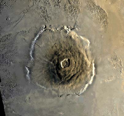
River Beds and Canyons
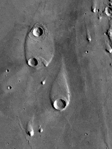
Martian Craters
Water and Life, Meteorites from Mars
The Martian Atmosphere
The Martian Satellites
Pathfinder-Sojourner
Summary
Lecture 25 - Mercury: A Moon-like Planet?
            2
         mV        GMm
        -----  =   ----
          r          r^2
Perihelion advance in sec per century
Planet     Predicted by        Observed
           Relativity

mercury      43.03              43.1
Venus         8.6                8.4
Earth         3.8                5.0

(Source: Bless, Discovering the Cosmos 1996)
Mariner 10
The Caloris Basin and Its Antipode
The Crater Kuiper
Crater Morphology
Surface Chemistry and Mineralogy
Polar Ice
Summary
Lecture 26: Venus
Like the Earth, But Not on the Surface
The Thick Atmosphere: Its Origin and Consequences
Earth's atmosphere with CO2 from Carbonates
Units 10^20 gm

oxygen         12.4
nitrogen       38.6
carbon dioxide 920
The Surface of Venus
                           0 Longitude
       --------------------------------------------
      |             *      MM      *               |
      |               * Ishtar    *      Atlanta   |
      |                  *  *  *                   |
      |   Beta                                     |
      |                                  ite       |
      |   Phoebe              A p     o d          |
      |                           h r              |
      |                                            |
      |                  L a d a                   |
      ---------------------------------------------
Summary
Lecture 27 - Transition to the Jovian Planets: The Asteroids
Astronomical Discovery
Eros and the Astronomical Unit
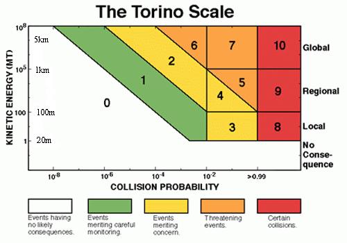
Orbital Families
      Table 27-1 a-Values for Orbital Resonance With Jupiter
m    n     a        m      n     a      m     n      a

2    3    3.970     3      4    4.295    4    5   4.489
2    4    3.278     3      5    3.701    4    7   3.583
2    5    2.824     3      7    2.957    4    9   3.030
2    6    2.510     3      8    2.706
2    7    2.257
2    8    2.065
2    9    1.909
The Failed Planet
Orbital Properties, Chaotic Orbits, Dinosaurs and Current Fears
The Nature of Asteroidal Bodies
Summary
Lecture 28 Second Hour Quiz - 8 November 2002
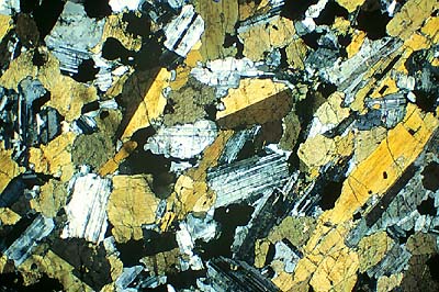
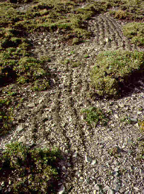
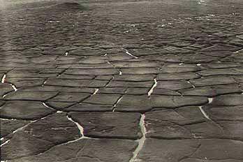