Models of the solar nebula may be calculated with the help of the thermodynamics discussed in Lectures 20 and 22. The classical calculations, developed along the ideas of Harold Urey, assumed that there was a unique temperature and pressure at each distance from the sun. Given these conditions, it is relatively straightforward to calculate the chemical and mineralogical composition of solids that are in equilibrium with the residual gas.
For realistic models, the gas is largely H2 throughout the nebula, with the usual admixture of 10% helium by number. We can set up a model starting with the SAD composition, and fix the temperature and pressure so that we get a density for the solid species at 1 AU from the sun of about 4 gm/cm3. This will match the uncompressed density of the earth. The models then show that water will condense out as ice a little beyond the asteroid belt. This is the location of the snow line.
In the inner solar system, the solids that have formed are essentially rock and metal. It is often thought that these solids are amorphous, ill or loosely formed. An essential point is that we do not really know how quickly these solids will collect to form bodies that can accrete. Collisions may be destructive as well as constructive, and we do not yet know how to fix the ratio between them.
Beyond the snow line, the solids that will come together are intrinsically softer, and perhaps they will have an easier time sticking together.
We are quite sure that the terrestrial planets have lost their complement of H and He from the SAD. Generally, strong winds from the early sun are postulated to have blown this excess gas away. The sun is then said to be in its T Tauri phase; the young stars named after the prototype T Tauri are known to have strong winds. However, if this gas blows past the outer solar system, it would also remove that gas, and consequently the Jovian planets could not form as we now observe them.
There are two possibilities. One is that the wind blows mostly out of the plane of the solar system. Perhaps there would have been enough wind to scour out the inner regions, but not where the Jovian planets are. This possibility is not usually considered. The more likely explanation is that the Jovian planets formed rapidly, before the energetic wind blew the nebula away.
It is generally believed that Jupiter and Saturn have substantial cores that are more like rock and ice in composition than the SAD. These rocky-ice cores are estimated to range from 5 to 15 times the mass of the earth. It is assumed these cores accrete, by much the same mechanism as the metallic-rocky terrestrial planets, that is, by constructive collisions.
There is a big problem here. The terrestrial planets can form on a relatively leisurely time scale, of the order of 107 or 108 years, after the residual gas of the solar nebula has been blown away. The giant planets must accrete much more material, perhaps 5 to 15 earth masses, before the gas has been expelled. Current calculations find a way to do this, but by setting adjustable parameters to favorable values.
We don't really know the distribution of sizes of accumulating planetesimals. Nor do we know the relative rates of constructive to destructive collisions--the fraction of the time when two planitesimals collide that a bigger body results rather than a smaller one. Within this blissful ignorance, we are free to set the parameters so we get the answers we need. We know the Jovian planets did form, and we have an idea of the time scale required for them to form. So we can take the existence of the planets as a way of fixing these unknown parameters. Some day, we may have a better way to do this.
A model of a planet is really a table of numerical values of thermodynamic variables as a function of radius. For our purposes, any physical system that has reached an equilibrium, or maximum entropy state may be described by two thermodynamic variables, plus the chemical composition. These two variables might be the temperature and the pressure, or the density and the pressure. The latter two variables turn out to be the most useful in practical calculations. We shall not worry about additional variables that may be necessary in a refined calculation.
The pressure at the surface of a giant planet is much lower than that at its center. It is a good approximation to assume that the surface pressure is zero, and increases toward the interior.
Consider an area 1 cm2 at the planet's surface,
and 1 cm in thickness--a cube, one cm on a side. If we
know the density of the material, we know the mass of the
cube. It is simply the density  times
the volume, 1 cm3, or just .
We assume this density has some small value, characteristic
of a value at the center of the cube.
Since we know the mass of the planet, M, we can compute
the force on the cube using Newton's law of gravitation.
Thus
times
the volume, 1 cm3, or just .
We assume this density has some small value, characteristic
of a value at the center of the cube.
Since we know the mass of the planet, M, we can compute
the force on the cube using Newton's law of gravitation.
Thus
         GM
F = ---------
          2
         R
Now this force, divided by the area at the base of the cube gives the pressure, P, since P = force/area. This gives us the first step in the creation of a model for the planet. We next need to have a way of estimating how much the density in the next cube down will increase as a result of the increase in pressure. This will enable us to take the next step in the construction of the model planet.
The new pressure thus requires a new density. Relations among thermodynamic variables, such as pressure and density are called equations of state. The simplest equation of state is that for an ideal gas, which we may write in several ways, e.g.
PV = nRT, or P =
RT/mu,
where "mu" is the molecular weight, and R the gas constant, 8.314 x 10⁷erg/mole/deg.
It is a good approximation to assume the equation of state is a perfect gas when the pressure is very small, and at that point, the molecular weight should be close to 2.0, for molecular hydrogen.
The model is constructed by requiring that at every level in the planet, the pressure is sufficient to support, or hold up the layers above it. When one gets to the center of the planet, the densities that have been calculated must be such that the known mass of the planet is obtained by adding all of the mass in the spherical shells from the center out to the surface.
Deeper in the planet, more complicated equations of state are required. What is the proper equation of state? This is the most important question for anyone who wants to make a model of a planet. Strictly speaking, we must know the physical conditions--the model, before we can give a valid answer. It would seem that we are in a hopeless situation, but in practice it is possible to make some progress. We proceed in a series of approximations.
First, we assume a very crude equation of state, and with its help, we get a first approximation to a model. The approximate model gives us an idea of the physical conditions, the thermodynamic variables for various points within the model. We can then formulate a better equation of state, and repeat the procedure.
If you have assumed the correct equation of state, then the densities at various radii will be such that all spherical shells will add up to give you the correct mass of the planet when you get out to the correct radius.
You can get the mass and radius to agree even if you have the wrong equation of state! This is the problem with science. You are never 100% sure you've got it right. What you can know for sure is that if your model doesn't give you the correct mass for the known radius, you've got something wrong.
Figure 29-1 shows the results of constructing models for giant planets under the assumption that they are pure hydrogen. The curve shows that for small masses, the radii increase with the mass. This is what one would expect for familiar materials.
Above masses of about 1031 gm, an increase of the mass results in a decrease of the radius. This happens because of the nature of the equation of state at higher pressures than are relevant for the planets. What happens is that the electrons are squeezed closely together, and quantum effects become relevant. We need not pursue this here. The phenomena are relevant for white dwarf stars.
Modern models of Jupiter have a dense, fluid molecular shell below the outer atmosphere. This material never liquifies in the sense of exhibiting a phase change, where the volume decreases virtually discontinuously with pressure. Indeed, for molecular hydrogen, there is a ``critical temperature'' above which this liquifaction is impossible. This critical temperature, 33K, is lower than any temperature of models of Jupiter, so that liquifaction in the usual sense of the word never occurs. Nevertheless, with increasing pressure, the gas density increases to values typically found in liquids, and it is common for workers in the field to use the term liquid to describe it. Strictly, it would be better to describe this material as a ``fluid,'' a term applicable to either a gas or a liquid. However, this refinement is often eschewed by workers in the field as well as writers of textbooks. At the relevant pressures, the hydrogen assumed metallic properties--it becomes a good conductor of heat and electricity.
You can see from Figure 29-1 that the points for Jupiter and Saturn come close to the theoretical curve for pure hydrogen, but those for Uranus and Neptune do not. You can see clearly that for the radii of the two outer planets, the masses are higher than those predicted for pure hydrogen models. This is the basis for the assumption that the Jovian planets have rocky cores. In the case of Jupiter and Saturn, the need for these cores is less demanding, but such cores are now assumed to be relevant for them also.
Stars and planets get divided into three zones, for good reasons. In the case of the earth, the three zones are core, mantle, and crust. The core is metal, the mantle is rock, and the crust is highly differentiated rock. The three zones for stars are called core, envelope, and atmosphere. Energy from the sun's core is transported outward by photons, so it is said to have a radiative core. Energy from the core is transported to the atmosphere mostly by convection, so the sun has a convective envelope.
The distinction between core, mantle, and crust seems appropriate for the terrestrial planets. Workers who model the Jovian planets tend to borrow the term used by the stellar workers, and call the thick, intermediate shell an envelope rather than a mantle. Both terms are in use.
In the envelopes or mantles of Jupiter and Saturn, the molecular hydrogen is squeezed first to a liquid, and finally to a metallic state. The corresponding zones of Uranus and Neptune are thought to have a larger component of rock and ice in their mantles than jupiter and Saturn.
Figure 29-1 shows that pure hydrogen models come close to the correct mass-radius relations for Jupiter and Saturn. Recall that the SAD is some 90% hydrogen, so these planets are probably mostly SAD on top of the rocky cores. These SAD envelopes probably formed by (rapid) gravitational collapse onto the cores. This is a mechanism used long ago to account for the formation of the stars from diffuse clouds of gas. If enough mass is present in a given volume, it will begin to collapse under its own self gravitation, that is, the outer layers will be pulled in by the inner regions. Since gravity is an inverse square force, the smaller the mass becomes, the greater the force pulling the outer layers toward the center.
Gravitational collapse will stop if the inner regions, the cores, can become hot enough or compact enough that high pressures stop the collapse. In stars, high temperatures stop the collapse. In the giant planets, it is stopped by phase changes, from gas to liquid or by the solid (rock or icy) cores.
Modern calculations have refined the picture of gravitational collapse, but the description remains qualitatively valid.
The outer Jovian planets, Uranus and Neptune, are smaller than the inner ones. It is not unreasonable to attribute this to the fact that they are at the edge of the solar nebula, and there was simply less material available.
In the next chapter, we will discuss in some detail the question of the heat balance in both the Jovian and terrestrial planets. Here, we will take up the question of internal sources of heat.
When the earliest space probes, the Voyagers, flew past jupiter and Saturn, they found both planets radiated more heat than they received from the sun. This was quite different from the situation that obtained for the terrestrial planets. What could the internal heat sources be?
In the case of the earth, it is possible to get a measurement of the heat flux coming from the interior. It is about 4 x 10¹³ Joules/sec, or 4 x 10¹³ watts. We can account for this flux by assuming that radioactive elements are decaying within the earth at known rates. There are other possibilities as well, so as far as the earth is concerned, we have an embarrassment of riches.
Radioactive decay cannot possibly supply the heat fluxes from the Jovian planets. It is generally assumed that the planets are either still shrinking, or that helium is sinking, causing the density at the centers of the planets to increase. Either of these possibilities could be considered primordial heat in the sense that it is derived from the same gravitational energy that was released as the planet formed.
The snow line is the zone beyond the asteroid belt where water would condense as ice from the solar nebula. The Jovian planets are thought to have begun as rock and/or icy cores in this region. These planets must have formed rapidly, before the early sun, in its T Tauri phase, expelled the excess gas of the solar nebula. Possibly the ices could coagulate more quickly than the metal and rocky materials of the inner solar system.
Jupiter and Saturn can be approximately fit by models consisting of pure hydrogen. They are mostly SAD in composition, with rock and icy cores. The intermediate zones, called envelopes (or sometimes mantles), probably formed by gravitational collapse. Rock-icy cores play a larger role in models of Uranus and Neptune. Their envelopes also contain a larger rock-ice admixture along with the SAD than their more massive congeners.
All four Jovian planets put out more heat than they receive from the sun. Radioactivity can not account for the excess heat. It probably derives from gravitation, but could also have a chemical source.
We have discussed the three modes of transport of energy, conduction, convection, and radiation. Heat is a manifestation of the energy of matter and radiation. In this context, radiation means photons, or light particles. Photons have energy and momentum, but no rest mass. There is no such thing as a photon with zero velocity. This, then, distinguishes radiation from matter, which may be in the form of electrons, protons, or neutrons. These particles may be in motion, or at rest.
The energy in any volume in space is a measure of the ability of the matter and radiation within it to do work. The second Law of Thermodynamics puts restrictions on the amount of work that can be done with that energy. We shall only make indirect use of those principles in this lecture.
We have seen that the energy of a molecule of a perfect gas is (3/2)kT. In general, ``kT'' is a reasonable measure of the kinetic energy of motion of an atom or molecule in a medium of temperature T. The constant, k, is called Boltzmann's constant, after the nineteenth century physicist, Ludwig Boltzmann.
Note that the gas constant, R (PV = nRT), is equal to Avogadro's constant (Na) times k. It is easy to see that if there are N particles in a volume, V, that N/Na = n, the number of moles. Thus the energy per unit volume, is (3/2)NkT/V = (3/2)nRT/V = (3/2) P. Thus we see that the pressure of an ideal gas is 2/3 of the energy density.
These relations for an ideal gas were well known by the end of the nineteenth century. Physicists also knew that radiation in equilibrium could be described by simple laws that depended only on the temperature, and not on the matter interacting with the radiation. It is essential for the radiation to be in equilibrium for this to be rigorously true. We can be sure that radiation and matter are in equilibrium if they are in an enclosure, and there has been time for all temperature inequalities to even out.
The english word for radiation that is present in equilibrium conditions is blackbody radiation. This word arose from experiments with radiation and soot-covered bodies, and is not especially descriptive. The corresponding german word literally means ``cavity radiation,'' and is a little more helpful. Radiation within a cavity is, by definition, blackbody radiation, provided the material within the cavity is in equilibrium.
One often sees the following definition: a black body is an object that absorbs all of the radiation (of all frequencies) that falls on it. Now if a body doesn't absorb radiation of some frequencies, it must reflect it. Indeed this property of matter can be very characteristic of its composition, and is the basis for reflective spectroscopy used in remote sensing (see Lectures 13 and 27).
A soot-covered ball absorbs most of the light that falls on it, and it emits a spectrum that is approximately that of an ideal black body.
The spectrum of an ideal black body follows a formula that contains mathematical and physical constants and one thermodynamic variable, the temperature. Some blackbody curves are shown in Figure 30-1. They are also called Planck curves, after the physicist Max Planck, who derived the mathematical formula that describes them. The relation is sometimes called the Planck Formula, or Planck's Law.
Both axes in Figure 30-1 are logarithmic. The smallest wavelength shown is 0.1 microns, or 1000 Angstroms. Note that the maximum of the curves shift to the left as the temperatures increase. Indeed, the wavelength where the Planck curves reach a maximum obey a simple relation:
 maxT = 0.29
The wavelength of maximum intensity,
max, is in centimeters, in
this formula, and the temperature in degrees Kelvin.
The total amount of energy that leaves unit area of a black body is directly related to the fourth power of the temperature (in Kelvin):
 T4.
T4.The constant is called Stefan's constant, or sometimes
the Stefan-Boltzmann constant. In cgs units,
= 5.670 x 10⁻⁵
erg cm2sec-1deg4. In SI units
= 5.670 x 10⁻⁸
watts meter2sec-1deg4. Remember
that a watt is a joule per second, or 107 erg/sec.
When radiation falls on any "non-(ideal)black surface," some fraction of the energy enters the surface, and the complementary fraction is reflected. The energy that enters the surface may be completely absorbed, or if the surface belongs to a thin layer, the energy that is not absorbed will be "transmitted." Most of the visible light that enters glass is transmitted. If the surface upon which light falls is thick, and opaque, we may safely assume that all light that is not reflected is absorbed. This is the situation with light received from the sun by planets, satellites, and asteroids.
The fraction of the light that falls on a planet that is reflected is called its albedo. There are several ways to define albedo, but we shall use it to mean the fraction of the total radiation that is reflected from a planet. Thus, if the planet receives an amount of energy E, from the sun, and the planet's albedo is A, then (1-A)E is absorbed by the planet, and AE is reflected into space.
Non-black surfaces emit radiation approximately according to
Stefan's law, but with a correction factor that is peculiar to
each substance, and to each temperature. The correction
factor,  , is called the thermal
emissivity. For soot, is very
close to unity, but for other substances, it can vary from
values near unity to values under 0.1.
, is called the thermal
emissivity. For soot, is very
close to unity, but for other substances, it can vary from
values near unity to values under 0.1.
Consider the planet Jupiter.
We can easily calculate the power that is intercepted by a disk
with its radius (RJ) at its distance from the sun.
The sphere surrounding the sun has an area of
4  r2, while the
disk of Jupiter represents an area
RJ2.
Here, r is the distance of Jupiter from the sun, and RJ
is Jupiter's radius. So the fraction of the sun's power
that is intercepted by this disk is
RJ2/(4 r2)= 2.1 x 10⁻⁹.
r2, while the
disk of Jupiter represents an area
RJ2.
Here, r is the distance of Jupiter from the sun, and RJ
is Jupiter's radius. So the fraction of the sun's power
that is intercepted by this disk is
RJ2/(4 r2)= 2.1 x 10⁻⁹.
The power of the radiation intercepted by Jupiter's disk comes if we multiply the above fraction by the sun's power output, 3.84 x 1026 Watts. The total power caught by the disk is 8.08 x 10¹⁷ Watts. This is not the full story because some fraction of this light must be reflected--otherwise we wouldn't see Jupiter. The fraction that is reflected is the albedo, and the figure we use for it is 0.70. This means 0.30 of the light falling on Jupiter is absorbed. Doing the multiplication, we get 2.4 x 10¹⁷ Watts.
We can use these concepts to estimate the temperatures at the
surfaces of all of the planets. The calculations are summarized
in the table below. What we do is equate the energy received from
the sun to the energy that would be radiated by a black body.
In the formula below, we assume the emissivity of the planet
is unity. Since it is more common to find planetary diameters, D,
in tables, we use R = D/2.
                        2
               \pi (D/2)                  2           4
(1-A) L(sun)x ------------- = 4\pi   (D/2)  \sigma x T        (1)
                       2
                4 \pi r
If we solve this equation for T, after calculating the energies received by the planets, we get the following predicted temperatures T = T(p), which are compared to measured temperatures T(m). In the following table, we give the distances r in astronomical units and the planetary diameters D in kilometers, as is done in the text. But for use in (1) all distances must have the same units. We must use meters, if we take sigma as 5.67 x 10⁻⁸ Watts per meter squared per deg4.
      Planet    Albedo    r       D      T(p)      T(m)
     Mercury    0.056   0.387    4878    441       440
     Venus      0.72    0.723   12102    238       250 (clouds)
     Earth      0.39    1.00    12756    246       280
     Mars       0.16    1.5237   6786    216       230
     Jupiter    0.70    5.203  142984     90       125
     Saturn     0.75    9.539  120536     64        95
The values T(p) in Table 30-1 are in reasonable agreement with the measurements, though not perfect. Planetologists often call this temperature, T(p), the effective temperature. This means nothing more than that a possible emissivity, that should be on the right side of Equation (1), has been set to unity.
All told, this technique does a reasonable job of predicting the surface temperatures of planets. We got fooled by the temperature at the base of the clouds on venus, but that is another story. We were fooled again, when the first probes, the Voyagers, flew by Jupiter and Saturn. These planets were putting out more heat than they received from the sun.
In order to see how this situation might arise, let us examine the sources of internal heat of planets.
The planets all have both internal and external heat sources. The most important external heat source now is the sun, but in the past meteoroid bombardment supplied a good deal of heat. Internal heat sources derive from radioactive decay, chemical energy, and gravitation.
The amount of energy released in a radioactive decay can be measured in the laboratory. The measurements are for specific, radioactive elements. In order to apply these measurements to the earth's heat supply, we must know the relative fraction of the radioactive elements in the earth.
The radioactive elements that are important heat suppliers are uranium, thorium, and potassium. Uranium and potassium have two naturally occurring isotopes. Both uranium isotopes are radioactive, though at different rates. Of the two potassium isotopes, only 40K is radioactive. To calculate the energy released from these two elements, it is necessary to know the abundances of the isotopes individually. Most calculations assume "natural" isotopic abundance ratios, values that can be measured in most substances. This is not necessary for thorium, where there is only one naturally occurring isotope, 232Th.
With the isotopic mixture of uranium and potassium, we can calculate the rate of energy generation, per gram, say of these elements. Note that Rb-87, which provides a very useful means of dating rocks is not an important heat source. It decays too slowly, and there is not enough of it.
The following table gives energy output rates for the important sources.
       0.97 x 10^{-7} Watts per gram of natural uranium
       2.7  x 10^{-8}  "     "    "  "  thorium-232
      36.   x 10^{-13} "     "    "  "  natural potassium
These figures as well as the ones following are from a 1988 book by John Verhoogen, ENERGETICS OF THE EARTH, that is often cited by geophysicists. The abundances are in parts per million (ppm) by weight. The first figures come from assuming the composition of the bulk earth can be estimated from the composition of certain meteorites. For potassium, the abundance is 170 ppm. To get the number of grams of potassium in the earth, we must multiply the 170 by the mass of the earth in grams 5.97 x 10^{27}, and then divide by a million. So the estimate is 1.015 x 10^{24} grams of potassium. To get the energy generated by radioactive decay of potassium, we now multiply by 36 x 10{-13}. If we do similar calculations for uranium and thorium, we obtain the following results.
   Source               Abund(ppm)      Power (Watts)
                                        (whole earth)

   Potassium            170             3.7 x 10^{12}
   Uranium               18 x 10^{-3}   1   x 10^{13}
   Thorium               65 x 10^{-3}   1   x 10^{13}
                                        -------------
   Total
2.4 x 10^{13}
The average heat coming from the earth's interior is estimated to be about 4 x 10¹³ Joules/sec, or 4 x 10¹³ watts. We can see that the radioactivities just about account for this output. Perhaps, because the abundances of these radioactive sources are themselves uncertain by as much as a factor of two, we may say the heat source is explained.
It is interesting, though to consider another source of heat, core
formation. Surely this was important at some point in the history of
the earth. In order to calculate this, we find the difference in the
potential energy of a sphere with a mean density of 5.5, with all the
mass distributed uniformly through it. This calculation is
done with a little calculus. Here, we just write down the answer:
               2
             M
PE = -0.6 G ----                                         (2)
R
Here, M is the mass of the earth, and R its radius. The factor 0.6 varies if the sphere isn't uniform in density, but it is nearly always close to unity (within 1/3 and 3).
We say the potential energy is negative, because we choose the zero point of the energy to be when the masses are all separated to infinity. We must put energy into the earth masses to effect that separation, so it's potential energy is negative.
G is the constant of gravitation. Notice that this is very nearly the potential energy of two masses M separated by a distance R. Now, let the mass be uniformly distributed in two layers, one with a density of about 4.3 (mantle) and another with a density of about 12.0 (core). Using the current dimensions for the core and the mantle, we find a mean density of 5.53, satisfactory for the earth.
If the earth were uniform in density, its potential energy would be
-2.24 x 1032 Joules. With a core, its potential energy
would be some 10% more negative. Consequently, we take the energy of
core formation to be about 2.24 x 1031 Joules. Now suppose
that energy were released over the 4.5 billion year lifetime of the
earth. The rate of release would be:
        2.2 x 10^{31} Joules
  ------------------------------------    = 1.5 x 10^{14} Watts (3)
  (4.5 x 10^9 years)(3.1 x 10^7 sec/year)
This is more by nearly a factor of 4 than the current power output of the earth! But we assumed that the core formation energy would be put out uniformly over the history of the earth. That cannot be true. Probably much of the power was dissipated early in the earth's history. It does seem possible that a small amount might contribute to the current output.
If we took the measured heat flux 4.0 x 10¹³ watts literally, and also the result 2.4 x 10¹³ watts from Table 29-3, we would need a little more energy.
Some additional energy may come from chemical changes. One may estimate the energy released per gram of iron, as it solidifies in the core. Other phase changes take place in the mantle. If we add all of these possible sources of chemical energy, we get only 1 to 10 per cent of that released by core formation. So we shall not consider these further for the terrestrial planets.
All of the quantitative concepts here basically use one formula: Amount = rate times time. We inverted this formula to get rate = amount divided by time. Can you point out which derivation used the formula in which way? The familiar formula distance = velocity times time is a special case of the more general formula, where "amount" is replaced by distance. Given any two of these quantities, you should be able to get the third.
Let us now turn to a discussion of the heat flow from Jupiter. Could this heat come from radioactive decay, as it does from the interior of the earth? We may test this hypothesis in the following way.
The power (energy per second) supplied by the dominant three radioactivities was given in Table 29-2. To see if we can get the Jovian heat output from them, we need only find out the masses of these three elements in Jupiter. This means, we need to know Jupiter's composition. Let us assume Jupiter has the same composition as the sun, what we have called the "solar mix" or the SAD --the standard abundance distribution. This isn't strictly true, but it is a reasonable first guess. If you click on the NEWS button on my HomePage, you can get the plot and a table of SAD abundances. In the astronomical convention, hydrogen is set at 1012, so its log is 12.0.
To estimate the mass of thorium in Jupiter, for example, we need the fraction of the mass of the SAD that is thorium, and then we need to multiply that by the mass of Jupiter. Since the SAD is given as numbers of atoms, we also need to consider the atomic weights. The average (atomic or) molecular weight for the SAD as a whole is 1.298. This is nearly the same as that of a mix that is 1 part helium and 10 hydrogen (about 1.27). The total number of atoms in the SAD is 1.098 x 10¹². The mass of the atoms in the SAD is therefore 1.425 x 10¹² grams.
To get the fraction that is thorium we need to divide this number into the mass of thorium in the SAD. The number of thorium atoms is 1.2, and the molecular weight of thorium is 232.04. So the fraction of the SAD mass that is thorium is 278.4/1.425 x 1012 = 1.95 x 10⁻¹⁰. We have to multiply this fraction by the mass of Jupiter, 1.9 x 1030 grams = 3.70 x 10²⁰ grams of thorium.
The final step in estimating the energy from thorium is to multiply by the figure given in Table 30-2 for the power from thorium per gram: 2.7 x 10⁻⁸. The result is about 1.0 x 10¹³ Watts.
We can proceed in exactly the same way for uranium and potassium. It turns out that potassium gives the major contribution, and the total for the three radioactivities is 5.5 x 10¹³ Watts.
The amount of heat emerging from Jupiter has been measured to be
                               18
Jovian power output = approx 10    watts           (4)
This is far more than could be supplied by the radioactivities--by more than 4 powers of ten. Consequently, there is no possibility that radioactivities could supply the heat that is currently coming from Jupiter. A similar situation holds for Saturn, Neptune, and possibly Uranus.
The amount of heat generated by radioactive decay within Jupiter is not far from the 4 x 10¹³ Watts coming from the earth's interior. Actually, this is not surprising. Although the mass of Jupiter is 318 times the mass of the earth, most of the additional matter is hydrogen and helium. Indeed only about 2% or 0.02 of Jupiter's mass is not hydrogen and helium. A good fraction of that 2% is in volatiles, carbon, nitrogen, and oxygen, lost to the earth. If we remove these elements from the SAD, the resulting mass is only about (1/300)th of the original. This is about the ratio of the terrestrial to Jovian mass.
No one has suggested that any substantial amount of heat is generated by chemical reactions in the Jovian planets. We are thus left with gravitation as the only plausible force capable of generating energy (force x distance).
The excess Jovian heat might be generated by gravitation in one of two ways. First, Jupiter might be in the process of forming a core with a density much greater than the bulk density of the planet. We have seen how this mechanism could work in the case of the earth.
Let us look at what might happen if something analogous to core formation on the earth happened on Jupiter. Consider the potential energy of two different density distributions. One is constant with planetary radius, and the other goes from some central value linearly to zero at the radius of the planet. Both calculations require calculus, so we'll just state the answers. For the constant density case, the potential energy is -0.6GM2/R, where M is the mass of the planet, and R its radius. In the second case, the potential energy is -0.7GM2/R; in the second case, the matter is a little deeper in the well. Let us take -0.1GM2/R as an estimate of how much energy might be released by density rearrangement. Neither of these simple density distributions is realistic, but their difference is probably a realistic (if rough) estimate of the energy that might be released by density readjustments in the real planet.
If we put in the figures for Jupiter, we find, using G
= 6.67 x 10⁻¹¹ Joule-meter / kg2.
SI units. Note a Joule-meter =
newton-meter2. Jupiter's mass must be in kilograms, and its
radius in meters to use this value of G.
  Estimate of energy from density distribution readjustment

         2                   -11           54
       GM          (6.67 x 10   )(3.69 x 10   )           35
 = 0.1 ----  = 0.1 ---------------------------  = 3.4 x 10   Joules (5)
        R                        8
                        0.71 x 10
This is the energy we have to work with. To turn it into a power, we
have to divide by a time. If we use the age of the solar system,
4.5 billion years, as we did for the earth, we find a power
(energy per unit time):
            35
    3.4 x 10                       18
--------------------     = 2.4 x 10   (joules/sec) or watts    (6)
        9           7
(4.5 x 10 )(3.1 x 10 )
This is fortuitously close to the heat output from Jupiter, which we have seen (Equation 4) is about 1018 watts.
It was originally suggested that the mass readjustment in Jupiter might be due to the heavier element helium sinking relative to hydrogen. But recent measurements of Jupiter's He/H ratio at the surface, from the Galileo probe indicated a nearly normal surface helium. By "normal" here, we mean the same as in the sun. Earlier estimates had led people to think that Jupiter's surface helium was below normal, and this could be explained if the helium had sunk relative to the hydrogen. This sinking would provide energy, as we have shown. Everything seemed to fit, and then an observation ruins the beautiful theory!! This isn't the first time this has happened in science.
The final chapter hasn't yet been written. Measurements of the H/He ratio in Jupiter's atmosphere do not necessarily apply to the bulk of the planet. Indeed, the parts of Jupiter's interior that are most important for the gravitational energy are deep within it. So we should not just throw out our beautiful theory. We just have to be cautious.
Most of the Jovian planets radiate more energy than they get from the sun. Here are some figures from a recent textbook:
                          Jupiter  Saturn   Uranus   Neptune
Energy from planet
-----------------          1.7      1.8      1.1       2.6
Energy from Sun
Observations of Saturn show that it has a helium deficiency. These are not as complete as those of Jupiter, but the sinking of helium is perhaps still viable for that planet. Don't bet a lot on it. Let us withhold judgement, and explore an even simpler scheme to get energy. Again, we take Jupiter for specificity.
Suppose Jupiter were shrinking, without necessarily changing the
density distribution within it. How much would it have to shrink
to provide the power, some 1.0 x 10¹⁸ Watts put out by
the planet? We can answer this with a calculation. The potential
energy depends on the mass and radius of the planet, along with a
constant factor, that depends on the distribution of density.
Usually, this factor, which we shall call
 (\gamma) is near unity. So we
don't need its exact value for a rough estimate.
(\gamma) is near unity. So we
don't need its exact value for a rough estimate.
Let us call the change in potential energy \Delta PE
( PE).
What is this change if the
radius of the planet changes by \Delta R (R).
This could be an
exercise in calculus. But we can just take the
difference of two expressions of the form of Equation (2).
In the first, the radius is R - minus a small increment,
\Delta R. The second term is the original potential energy.
PE).
What is this change if the
radius of the planet changes by \Delta R (R).
This could be an
exercise in calculus. But we can just take the
difference of two expressions of the form of Equation (2).
In the first, the radius is R - minus a small increment,
\Delta R. The second term is the original potential energy.
                           2                       2
                         GM                      GM
\Delta PE = -\gamma  --------------   +  \gamma ---------    (7)
                     (R - \Delta R)               R
The first term on the right of (1) is bigger in absolute value, that is, more negative, than the second, because we are dividing by a smaller number. The numerators are the same, and we assume the \gamma's are the same too--similar density distributions.
We can get a power from (1) by dividing the energy by a time interval. Evaluation of the right-hand side is an exercise in the manipulation of small quantities. We assume \Delta R << R, and use 1/(1-x) is about equal to 1+x if x is small. I'll let you work out the details, as for this course, we are only interested in the result. We want to divide the difference in potential energy by a relevant time increment, which we shall call \Delta t. Then
                        2
\Delta PE             GM      \Delta R
---------   = \gamma -------  --------                (2)
\Delta t                 2    \Delta t
                       R
The (\Delta R)/(\Delta t) is a distance increment over a time increment, that is, a velocity. What we want to know is, how large must that velocity be for the power output (\Delta PE)/(\Delta t) to be 1.0 x 10¹⁸ Watts. We know all of the quantities in (2) on the right hand side except for the (\Delta R)/(\Delta t). So we equate them to the current power output of Jupiter, and solve for the unknown. With \gamma = 1, we find that (\Delta R)/(\Delta t)= 2.1 x 10⁻⁹ centimeters per sec!! is all that the rate of shrinkage needs to be to supply the current power output. That rate would not be detected by any measurements currently available.
In the roughly 500 years since Jupiter has been under telescopic observation, it would have shrunk by 2.1 x 10⁻⁹ (cm/sec) x 500 (yr) x 3.1 x 10⁷ (sec/yr) = 33 cm. That is only about 2 parts in 108 of the radius of the planet. The radius of the planet cannot be uniquely given with that accuracy, since the atmosphere is gaseous.
We conclude Jupiter could derive its power either from simple shrinkage or a density redistribution. The density redistribution is now thought to be more relevant for Saturn.
Energy from the sun in the form of radiation falls on the disks of the planets. Because they are not perfect black bodies, some fraction of this energy is not absorbed. The fraction is called the albedo. We can account roughly for the surface temperatures of the planets by equating the solar influx times (1 - albedo) with the output from a black body with a temperature called the ``effective temperature'' of the planet. The Jovian planets put out more energy than they receive from the sun.
The energy flux from the earth's interior can be accounted for by the decay of radioactive elements uranium, thorium, and potassium. These sources are not sufficient for the Jovian planets. Gravitational energy does seem to be an adequate source for them. It could arise either from a redistribution of the planetary masses or a simple shrinking of the planets' radii.
In Lecture 12, we discussed a set of four equations developed in the nineteenth century, and now known as Maxwell's equations, after their originator, James Clerke Maxwell. These equations described scalar quantities, electrical and magnetic ``charges'' (see below), and vector quantities, the electrical and magnetic fields. Recall that a scalar quantity, like temperature, can be described by a single number, but a vector requires three, since it has both a magnitude and a direction.
One of the intriguing aspects of Maxwell's equations, is that isolated magnetic ``charge'' does not exist. By contrast, isolated electrical charges are familiar. On a microscopic scale, we may have isolated positive or negative charges, protons or electrons. On larger scales, a net positive or negative charge may reside on some macroscopic object, which can be isolated in space. No similar analogues are known to exist for magnetic charges.
Magnetic fields, on the other hand, emanate from poles of a magnet. These poles are called N and S, or + and -, the latter, rather like electrical charges. The big difference is that no one has ever located an isolated magnetic pole. All known electrical and magnetic phenomena seem to be adequately described without one.
How could you tell if there were such a thing? Here's one way. Suppose you had an isolated bit of electrical charge, which for purposes of argument, we'll say was positive. Consider a sphere of some fixed radius that surrounds the charge. We'll suppose the sphere is much bigger than the charge itself. If we took another positive charge and put it anywhere on this sphere, it would be pushed away from the center of the sphere.
Now let's try the same trick with a magnet. The only magnets we know have two ends, they are dipolar. But we can imagine a very long magnet, and surround its N pole with a sphere. The sphere can be big, but the magnet's length must be greater than the sphere, since we are trying to isolate one pole.
Finally, take (in your imagination) another long magnet, and poke the N end of it all around the sphere that surrounds the first. What every experiment finds is this: While the N pole of the second magnet will be pushed away from the center of the sphere at some points, there will be others for which it is pulled toward the center.
Lines of force give the direction a charge (pole) would be pushed by the field of another charge (pole). If there were an isolated charge, one could surround it by a sphere, and all of the lines of force would leave (or enter) the sphere. This never happens for a magnetic pole. In fact, one of the Maxwell equations states that the net magnetic lines that go into and out of any closed volume will always balance. This also happens for electrical lines of force, provided there is no charge within the volume.
Some exotic theories of physics have postulated the existence of isolated magnetic charge, called magnetic monopoles. These monopoles play a role in some theories of the early big bang. As of this writing, there is no evidence that monopoles manifest themselves in the world in which we live.
Magnetic fields can be generated by electrical currents. Even the fields that exist in natural magnets can be thought of as due to tiny currents within atoms. They arise due to what is called the electron spin, but we won't go further into this topic.
A long wire conducting an electrical current will be surrounded by rings of magnetic field lines. This can be tested with a small compass needle. If you turn the current off, the magnetic field will collapse.
There is energy in a magnetic field. If you have a current flowing in a wire loop, there must be a magnetic field about the wire. Then if you break the current with a switch, and the field disappears, what happens to that energy? How does it manifest itself? You can do a simple experiment to show that if you just barely open the switch, a spark will jump across it. In other words, something will make the current try to continue to flow. The energy to do this, it turns out, comes from the collapsing magnetic field.
There is also energy in an electrical field. We have seen in Lecture 12 that photons, particles of light, are manifestations of both electrical and magnetic fields. The energy of photons may be thought of as coming from their associated electrical and magnetic fields.
Electric fields by definition exert forces on charges. Charges in motion give rise to electrical currents. These currents can discharge the fields, so they no longer exist. Suppose we painted one wall of a room with positively charged paint, and painted the opposite side with an equal amount of negative paint. This would create an electric field in the room, since a positive charge in the middle of the room would be pushed away from the positive paint, and pulled toward the negative paint. However, if we filled the room with mercury (which conducts electricity), the field would quickly discharge. All of the electrons in the negatively charged paint would flow through the mercury and neutralize the positive wall.
Since there is no such thing as a magnetic charge, there is no magnetic phenomena that quite corresponds to the example of the painted room. There is no magnetic analogue of an electrical current. In cosmic phenomena, there is often no simple route to the destruction of a magnetic field.
We have seen, in the case of a simple current loop, that magnetic fields are certainly destructible, but the simple route of discharge (equalization) is not open to them. Electrical discharge can take place through a conducting medium-- one capable of carrying current. It turns out that most of the cosmos--plasmas--is rather highly conducting, and this means that strong electrical fields rarely occur. The absence of magnetic currents has the consequence that there are many manifestations throughout the cosmos of magnetic fields and associated phenomena. In this lecture, we shall explore some of them.
We saw in Lecture 13, in connection with the discussion of the mass spectrograph, that a charge moving in a magnetic field would experience a force. The force is perpendicular to both the direction of motion of the charge, and the field. In a medium with a high electrical conductivity, this force has the effect of binding the matter to the field, or vice-versa. Depending on the strength of the field, the matter will either be bound to the field, or the field will be transported by the matter.
It is common to describe this situation by saying the magnetic field is frozen into the medium, although this is strictly true only for material motion perpendicular to the field direction. Flow along the field direction is not inhibited. If the energy of motion of the medium is larger than the energy in the field, motions of the medium are capable of moving the field in such a way that it becomes either stronger or weaker.
One useful measure of the strength of a magnetic or electric field is the number of lines of force through a unit area. The field can be doubled by doubling the lines of force through some area. If the field is frozen in a medium, it may happen that the fluid motions are such that the magnetic field is twisted round on itself so that the lines reinforce one another. This is illustrated in Figure 31-1 for a ``loop'' of magnetic field.
(see drawing from lecture)
You can do a simple experiment yourself with a rubber band. First mark arrows along it to indicate a direction for the field. next, form a figure eight, and twist the band back on itself. You will see that the arrows will again line up, but where there was once one strand of the band, there are now two. Just as the strength of the band has doubled, a magnetic field will double in strength if it is pushed in this way by the motions of a conducting fluid medium.
Of course, you can also simply take the two ends of the rubber band and stretch them, until the arrows going one way are very close to the arrows going the other. In this case, there would be no net flux, and the field would essentially have destroyed itself.
We believe that motions in the liquid core of the earth act in the former of these two ways, to build and maintain the earth's field. The overall mechanism of building a field is called the dynamo mechanism--the same name that is used to describe a generator of electrical current.
We do not know in detail how the earth's dynamo works, nor are we sure why the field is built up rather than weakened, as in one version of our experiment. One possible explanation postulates that it is natural for energy to distribute itself among its possible manifestations. This means for mechanical energy, that kinetic and potential energy would tend toward equality. For systems obeying Newton's laws, this is generally the case.
If the same principle applies to the magnetic energy, and a conducting fluid, with the field frozen in. Then if there were originally strong fluid motions, and weak magnetic fields, the motions would be such as to strengthen the fields. When the energy in the field and in the fluid motions were comparable, the field strengths would cease to grow.
The strength of the earth's magnetic field varies somewhat, with position on the surface. Roughly, it is one to ten thousand times less than a strong bar magnet, ample for the operation of a compass. There are two relevant ways to give the relative strengths of planetary magnetism. Table 31-1 gives magnetic field strengths at the surfaces of the planets relative to the earth's surface field. Also given is a measure of the strength of the magnets that would simulate the planetary fields if they were placed within the planets. (This ``strength'' is called the magnetic moment.) The two columns of the table differ by the cube of the radii of the planets.
            All Field Measures Relative to Earth

          Mean Surface    Magnetic Strength   Angle of pole to Axis
              Field        (dipole moment)    of Rotation (degrees)

mercury        0.011        6 E-4*                ?
venus         <0.001       <8 E-4
earth          1.0          1 E0                  12
mars          <0.002       <3 E-4
Jupiter       13.8          2 E+4                -10#
Saturn         0.6          5 E+2                  0
Uranus         0.7          4 E+1                 59
Neptune        0.4          2 E+1                -47

* The number following `E' is the power of ten that
should be applied.  Thus 6 E-4 means six times ten
to the power minus four.
#This indicates the NS direction of the dipole is opposite
that of the earth.
Roughly speaking, the fields of the equivalent magnets for the planets are shaped about like the fields of a bar magnet. However, important modifications from this shape occur as a result of pressure from the solar wind, which squeezes the field on one side of the planet, and causes a kind of tail on the other.
Fast, charged particles from solar storms or flares travel outward through the interplanetary medium. Some of these particles will interact with planetary magnetic fields. The nature of this interaction is basically the same as that discussed in Lecture 13. The charges experience a force that is perpendicular both to the field, and to their velocity. This makes them spiral around the field lines.
The volume of space where a planet's magnetic field significantly influences the motion of charged particles is called the magnetosphere. This is a simplified concept, since there is no sharp boundary between regions of space where the trajectory of a charge is influenced and one where it is not. Generally speaking, particles which enter a planetary magnetosphere move along the lines of force. These lines of force typically end on the planetary surfaces near the magnetic poles.
We see the effects of these charged particles when they collide with atoms in the earth's atmosphere. The atoms are excited by these collisions--they absorb energy. This excess energy is radiated away in the form of photons, which may be seen from the ground as aurorae. The most common auroral lines are red or green, and are due to transitions in the neutral oxygen atom.
The magnetic fields of the Jovian planets give rise to aurora that have been seen on all four of them. Important work on these phenomena have been done at the U of M by John Clarke and his colleagues at the Department of Atmospheric and Oceanic Sciences. They have obtained impressive images using the Hubble Space Telescope. (Type "aurorae" into a search engine.)
One of the more spectacular interactions takes place between Jupiter, and the inner Galilean satellite Io. As the satellite moves through the ionized medium between it and Jupiter, electrical currents are generated that follow the magnetic field lines between planet and satellite. The effects of these currents are sometimes manifested as aurorae on Jupiter. Currents were actually measured by the 1979 space probe Voyager I.
Only a few minerals are strongly magnetic. Run a magnet through beach sand, and you will quickly find that most of the black grains are strongly magnetic. These grains are mostly magnetite, Fe3O4 (cf. Lecture 23). But you will also find that other grains are attracted to the magnet.
The inherent magnetism of a solid like a rock or mineral depends (interestingly enough) on its history. If the material contains atoms, like iron or nickel that have partially filled inner electron shells, then each atom can act like a little magnet. The magnetism arises ultimately from the spins of the electrons. A grain of material will act like a magnet if the individual atomic spins have some net alignment.
In the case of materials like magnetite, the atoms will align naturally, forming a natural magnet. Other materials can exhibit what is called induced magnetism by placing them near a strong magnet.
Materials will lose their magnetism if they are heated to a high enough temperature. The critical temperature is called the Curie temperature, or Curie point. In general, the Curie temperature is lower than the melting point, so that any igneous material may safely be assumed to have passed through a state of no magnetization (liquid) to one where magnetization is possible.
What will be the direction of the field of magnetic igneous materials? Generally speaking, those materials will preserve the field direction of the earth at the time the temperature dropped below the Curie temperature. This provides the geologist with an interesting way of determining the history of planetary magnetic fields.
We can read the history of the earth's field near the mid atlantic ridge, where ocean floor is constantly being created, and pushed east and west. We discovered in the 1960's that the magnetic pattern was striped, with the average polarity of the rocks of the ocean floor alternating with distance from the ridge. This observation actually cinched the theory of plate tectonics, as well as providing a detailed record of the history of the earth's polar reversals.
For reasons that are unclear, the earth's magnetic pole reverses direction on a time scale of the order of half a million years--short. We do not know what causes these reversals, but the evidence for them is very clear, and can be read in the general geological column (cf. Grand Canyon Layers) as well as in sea floor spreading.
We have yet to exploit the magnetism of planetary materials beyond a few cases. Lunar rocks show evidence of a slight magnetism, whose origin is puzzling, since the Moon now has no general field. Did it have on in the past, or were these rocks somehow magnetized by the solar wind?
We have discussed the magnetic field of the sun (Lecture 6). The origin of this field is not entirely certain. The original field may have come from the interstellar cloud from which the sun formed. We now think this field is strengthened and maintained by a dynamo mechanism that is driven by the differential rotation of the sun-- low latitudes rotate more rapidly than the higher latitudes.
It is now known that magnetic fields exist throughout interstellar space. Indeed, our Galaxy is threaded by such fields. Even though typical interstellar fields are quite weak, they play an important role in many cosmic phenomena.
The famous equations of Maxwell tell us that magnetic fields may be generated by electrical currents. At the present time, we do not know the nature of the currents that generated most of the cosmic magnetic fields. We have discussed a simple dynamo mechanism that will build up a magnetic field that is threaded through a conducting medium. It was necessary for us to postulate that the medium moved in the proper way to strengthen the field. We could give only a rather general, plausibility argument why this might happen.
The term fossil field is often used to describe a field whose origin is uncertain. The notion of a fossil field is often used when one is willing to accept the existence of a field due to unknown causes. Given the presence of a field, it is possible to work out some of its consequences. For example, given the general magnetic field of the galaxy, we may investigate the effect on star formation in giant molecular clouds.
In principle, the answers to many of our questions lie in Maxwell's equations. Unfortunately, it is not possible to give a general solution to these equations--the kind of solution that is available for the two-body problem, or the falling body problem. We can only make models, and use the equations to try to follow their subsequent behavior. Computers are only now getting the necessary speed and memory to attack such problems.
Maxwell's equations tell us that magnetic fields may be generated by electrical currents. The earth's magnetism is manifested in a large variety of ways from compass deflections to aurorae to the magnetic stripes of the mid-Atlantic ridge. We think the earth's field is maintained by a dynamo mechanism. We understand in principle how it might work, but we do not know the detailed mechanism. Magnetic fields are frozen in highly conducting media, and those motions are capable of generating or strengthening the fields. The Jovian planets all have magnetic fields, and have aurorae. These are caused by the interaction of particles from the sun with the local magnetospheres.
There are many manifestations of a general interstellar magnetic field in our Galaxy. It acts to constrain the cosmic rays, and provides support through its magnetic pressure to giant molecular clouds. Some stars, and especially white dwarfs and pulsars have very strong magnetic fields.
Jupiter is surely the dominant planet of the solar system. It's mass is nearly three times that of its nearest rival, Saturn, and more than 300 times that of the earth. If we take Neptune as marking the edge of the planetary system, then Jupiter is only 20% of the way out to it. However, in terms of the mass in the solar nebula, Jupiter could have been closer to the halfway point. By this, we mean that the mass in the original solar nebula within 5.2 AU could have been half of the total mass of the nebula. This is because we think the density of the nebular gas would have been higher closer to the sun.
We do not know the conditions in the early solar system, of course. We make models, and follow their evolution with computers. Some of these models show considerable migration of the planetesimals from the inner to the outer solar system. Perhaps Jupiter was once much closer to the sun than it now is. We shall see in Lecture 37 that some extrasolar planetary systems have giant planets closer to the central stars than we ever thought would be possible.
We know a good deal about today's Jupiter. We discussed the Hubble Space Telescope's observations of the Jovian aurorae in Lecture 30. The HST and space probes, especially Galileo, have provided detailed pictures of the complex patterns of flow that have developed in Jupiter's atmosphere. The simplest aspects of this flow have been known for some time. Energy from Jupiter's interior is transported by convective currents. Jupiter is rotating quite rapidly, once about every 10 hours, and this rotation distorts the convection cells into a system of belts and zones.
The Galileo probe confirmed that the atmosphere is undergoing convection, the transport of hot gas from below to cooler layers above it. In Jupiter, this gives rise to the bright zone, dark belt structure. Idealized structure is indicated below. We'll only show the southern hemisphere. Nomenclature for the north is the same, only with the word South replaced by North. Assume the surface rotates from left to right --->
--------->-------->----------->-----------------x
Equatorial zone                                  x
-------->--------->----------->---------------- x
South equatorial belt                           x
--------<---------<-----------<----------------x
South tropical zone  (Great Red Spot)          x
-------->--------->----------->---------------x
South temperate belt                         x
--------<---------<-----------<-------------x
South temperate zone                       x
-------->--------->----------->----------x
South South temperate belt              x
--------<---------<-----------<------- x
South South temperate zone           x
                                   x
                                x
                              x
                            x
South Polar              x
Region                x
                  x
           x
x
The bright zones represent hot material rising, and the dark
belts, material sinking. Let us see how this
gives rise to a flow pattern. The concept
we need for this is just that the matter near the equator is
rotating about Jupiter's axis faster than that at points between
the equator and the poles. At the poles, there is no velocity due
to the rotation, of course. For any intermediate latitude, the
velocity of rotation is
(2R)/(Period of Rotation), where R is
the distance from the axis of rotation to the surface of the
planet--something like the dashed lines in the figure above.
Rising material from the equatorial zone that moves north is going faster than that the surface under it. A similar thing holds for rising material that moves south. So the flow arrows on both the north and south edges of the Equatorial Zone point to the right (which is the assumed direction of rotation of the planet).
Material flowing from the South tropical zone into the South equatorial belt (thence down) is going more slowly than the material of the belt, because the belt is closer to the equator. Hence the flow pattern is to the left. Material from the South tropical zone that flows (south) into the South temperate belt (thence down) is deviated to the right, because the South tropical zone is going faster than the South temperate belt (to its south).
Check the lectures for a diagram. If there is time, I'll put one up here.
(see lecture for drawing)
The envelopes of Saturn, Uranus, and Neptune resemble that of Jupiter, though not in detail. We will not describe them separately.
The heat output from Jupiter may have influenced the densities of the bodies that formed near it, in particular, the Galilean satellites. Here are some figures. The ages of the surfaces are determined from crater densities.
Object                   Io      Europa     Ganymede    Callisto     Mercury
Density (water=1)        3.5      3.3        1.9         1.8          5.4
Composition              rock    rock      rock+ice     rock+ice    Metal+rock
Diameter(km)             3630    3128       5262         4800         4878

                              8         8          9         9            9
Age of surface (yr)   few x 10  few x 10   3.5 x 10    4 x 10       4 x 10
Of the Galilean satellites the innermost Io is still active, with volcanos and lava flows. Most of the craters on its surface have been covered. The energy that drives this activity comes from tidal interaction between Io and Jupiter. While Io is some 5.8 Jovian radii away, it is only slightly over twice the Roche limit (see Lecture 31), and is therefore subject to strong tidal forces. We think that the orbit may have been more eccentric in the past, and this would have enhanced the tidal heating.
Europa is not now active, but must have been so in the not too distant past. Its crater density is quite low. Recent images of the surface of Europa suggest that there have been extensive outflows of water from its interior. It is possible that some tidal heating has been sufficient to maintain a zone of liquid water within the body. We shall soon discuss why the presence of liquid water always raises the possibility of life forms.
By contrast with Io and Europa, Ganymede and Callisto are heavily cratered.
Possibly the heat from Jupiter, during the formation of the satellites accounts for the density decrease, from inner to outer. Certainly, this mimics the densities of the planets themselves. This is still an open question.
It is entirely possible that the tidal heating drove off an icy fraction of Io, either when it was forming or afterward. Perhaps to a lesser extent, the same thing happened with Europa. This might account for the high densities of these inner satellites, without invoking the heat from the central body. In much the same way, some people have attempted to account for the density gradient of the planets by ad hoc (special) causes. Mercury, they say, is dense not because the rocky component could not form at its position, but because it was blasted away, after the core had formed.
The Jovian planets have lots of satellites. The 1998 Astronomical Almanac lists 16 for Jupiter. We have discussed the major, Galilean satellites of Jupiter. These have radii of some 1500 to 2400 km. Thus, they are relatively large bodies, ranging in size from slightly smaller than our own Moon to about 50% larger.
The remaining Jovian satellites are all an order of magnitude (or more) smaller. Four of these small satellites are nearer to Jupiter than Io. Their orbits, like the Galilean satellites, are closely confined to Jupiter's equatorial plane, and their eccentricities are very small. Generally speaking, interactions of accreting satellites, collisions among the fragments, are expected to circularize the orbits and to confine them to the equatorial plane of the planet. This happened not only for the Galilean satellites, but for four smaller inner satellites.
Outside of Callisto, the outermost Galilean satellite, we could group the satellites into two categories. There is a group of four, some ten times the distance of Callisto from Jupiter. The orbits of these four show a definite ``relaxation'' of the close coupling to Jupiter. They are somewhat eccentric, and somewhat inclined. Another set of four satellites is about 20 times further than Callisto. All four have retrograde orbits--they revolve opposite the direction of the inner satellites. Speculations are that the outer four satellites, and perhaps the outer eight were captured by Jupiter.
Saturn has 18 satellites listed in the Astronomical Almanac. Only one of them, Titan, is comparable in size to the Galilean satellites of Jupiter. This satellite has an atmosphere, mostly of nitrogen gas (N2),with small admixtures of argon, methane, and hydrogen. Only one of the 18 satellites orbits retrograde, but some of the outer satellites show modest eccentricities and orbital inclination. They have either been perturbed or perhaps captured.
Uranus is the fascinating case, because its axis of rotation is tipped more than 90o to the pole of the ecliptic. We could say the planet rotates in a retrograde sense, but the angle of the polar axis to the plane of the ecliptic is only about 8 o. The rotation axis is almost in the plane of the orbit. We call upon the planetary deus ex machina, the collision, to account for this strange rotation, just as we must in the case of venus. Somehow, 15 satellites knew to line up in the tilted equatorial plane of the planet. Presumably this means the satellites formed after the putative collision that affected the rotation.
Neptune has eight satellites. The two outermost ones have clearly disturbed orbits. The outermost, Triton is about 20% smaller than our Moon. It's retrograde orbit was once the basis for speculation that Pluto was an escaped satellite of Neptune. The two objects are of comparable size. Nereid is about one tenth the size of our Moon. It's orbit has the highest eccentricity of all the satellites, and its semimajor axis is larger by more than 10 than that of Triton. Surely these satellites were either captured, or their orbits were severely perturbed by some large planetesimal.
Energy from the interiors of the Jovian planets is carried by convection. At the surfaces of the planets, convection currents manifest themselves in bright zones of rising material, and dark belts of sinking material.
The Galilean satellites of Jupiter show a density decrease that might be due to heat from the planet, though this is not certain. Io is currently active, and Europa may have been active recently. It may also still have liquid water below its surface. Ganymede and Callisto have very old surfaces.
The satellites of Jupiter and Saturn fall into two categories, inner and outer. The inner ones all have very low eccentricities, and orbital inclinations. The outer ones have larger eccentricities as well as inclinations. In addition, the outer ones may orbit in a retrograde fashion. The outer satellites may be captured asteroids.
Satellites of Uranus are generally constrained to the plane of it's tipped equator. Their orbits are generally ``well behaved,'' that is small inclinations and eccentricities. Neptune has four well-behaved inner satellites and two outer ones with highly perturbed orbits.
Until the space age, the only planet that we knew had rings was Saturn. The rings were poorly, though definitely seen in Galileo's crude telescopes. These rings can be clearly seen in good quality telescopes of small aperture, but the images are small and often disappointing. Larger telescopes, say 30 inches or more in aperture, provide quite breathtaking views of Saturn, but these telescopes are usually available to the public only at the times of ``open houses'' at observatories. Beautiful telescopic photographs of Saturn, many in color, appear in popular and textbooks on astronomy. The first Saturn fly-by's, the Voyagers (1979), returned many images of Saturn's rings as well as some of its smaller satellites. Many new aspects of the ring system were seen, and some presented interesting challenges to the astronomer to account for them.
Jupiter, Uranus, and Neptune, all have ring systems. Jupiter's ring was discovered by the Voyager mission. The rings of Uranus and Neptune were discovered by ground observations, but confirmed by the Voyagers.
The nineteenth-century French astronomer Edouard Roche (1820-1883) provided a general explanation for ring systems. He was able to show that small bodies within a certain distance from a planet would not be able to grow in size because of tidal forces. The critical distance is now known as the Roche limit.
Consider the following question. Suppose there are two spherical masses 'm', in contact with one another, and lined up with the center of a much larger mass 'M'. Let the distance of the first little mass from the center of the large one be 'd', and let the radii of the little masses be 's'.
What will the distance d be such that the difference in the gravitational force on the inner and outer small mass is equal to the gravitational attraction of the two masses to one another?
.(see figure from class)
.
.
.
.
.
.
.
.
We can write this out:
Force     Force of planet  Force of planet
between   on closest       on outer
2 masses  little mass      little mass
  |          |                |

Gmm         GMm              GMm
-----  =   ------     -     -------         (1)
    2         2                    2
(2s)         d               (d+2s)
The difference in the forces on the right-hand side of (1) is a tidal force. Some algebraic manipulation, along with approximations when 2s << d show that the tidal force depends on the inverse cube of d. Thus the tidal forces increase rapidly when d gets smaller. Equation (1) allows us to find the border where the tidal force and gravitation are just in balance.
Let us assume that the densities
() of the large and small
masses are the same. Then it follows from (1) that the tidal and
gravitational forces are in balance when
 d
--- = 2.520...              (2)
 R
where R is the radius of the mass M. The distance 2.5R is known as the Roche limit. If the distance is less than 2.5R, tidal forces would not allow a body to be held together by gravitation.
None of the major satellites revolve around their parent planets within this Roche limit, but all of the ring systems do. We therefore conclude the rings did not form because of tidal forces.
Tidal forces do not tear the Space Shuttle apart--why? The answer is that the Roche limit only compares tidal forces to gravitational ones. Gravitational forces are much weaker than chemical forces which are responsible for the shapes of objects we are familiar with. On the other hand, if we compare chemical and gravitational forces for large objects, the story is different.
Consider a square block of matter that we can conceptually divide in
half. If each side of the block is s, say, then one half of the
block will attract the other gravitationally with a force that is
equal to Gm2/s2.
There is a factor , that
depends on the geometry. If we took two balls in contact, then
would be a little different than for blocks.
We will just set = 1,
here. It is of order unity, and
it's exact value will not affect our argument.
                  --------------------------      Cross section
                  |           .            |      of a block of
                  |           .            |      material.  Dots
                  |   m/2     .    m/2     |      represent a plane
                  |     x<-- 0.5s-->x      |      dividing one half
                  |           .            |      of the block from
                  |           .            |      the other.
                  |           .            |
                  --------------------------
                  <------------s------------>
What are the chemical forces that hold one half of the block to the other? There will be some chemical force per unit area that depends on the nature of the substance. The total chemical force will be related to the number of atoms or ions on the left surface that attract those on the right surface of the contact plain, indicated by the vertical dots. The total chemical force holding the halves of the block together will depend on the area. That area depends on s2. We can actually make a rough estimate of how strong these forces are, because we know the strengths of typical chemical bonds. Let's save this exercise for the moment.
The masses m/2 depend on s^3 and a density. This means the gravitational force will depend on s6/s2 or s4. The ratio of the gravitational to the chemical forces in any body thus depend on s4/s2 or just s2. So the bigger the body, the more important the gravitational force.
Remember the four forces of nature. Gravitational ones are the weakest. Electromagnetic forces, which are basically what chemical forces are, are much stronger. But for bigger and bigger bodies, there will come a time when gravitational forces are more important for the body as a whole. Locally, chemical forces will always be more important.
Bodies in the rings are thought to be no larger than some tens of meters across. So this must be about where gravitational and chemical forces are in balance for the material in these ring systems. There is a distribution of sizes from the maximum (tens of meters) down to dust.
A question that is related to the concepts of the Roche limit is the following: A at what point gravitational forces make cosmical bodies round. That turns out to be a much larger size, of the order of 10 to 100 km or so. Small satellites and asteroids are lumpy, large ones are round. After the mass of an object is sufficiently large, the gravitational forces simply crush the material into a spherical form. The reason for this is that the sphere is the geometrical figure that contains the greatest volume inside the smallest surface area.
The Voyager space probes revealed a more complicated ring system than had been seen from the ground. Photographs from earthbound telescopes typically show two rings, called A and B. The gap between the A and B ring is named after the astronomer Cassini, and is called Cassini's division. The A ring is itself divided by a less prominent gap known as Encke's division.
Cassini and Encke were both important figures in the history of astronomy. Cassini (1625-1712) was a contemporary of Newton. Perhaps his most important contribution to astronomy was the determination of the distance to Mars, which was for many years the basis of the astronomical unit (Lecture 4). Encke was nineteenth century, and may best be known for the discovery of a bright comet that bears his name.
Inside of the B ring, there is a C ring (dark in Figure 32-2) and a D ring. These, and outer rings are not usually seen from the earth, but they do show up on Voyager images. Indeed, the Voyager images show so much structure within the rings, and even in Cassini's division, that the traditional names are not particularly descriptive. These images also showed markings or shadows on the rings themselves. Some of these features have been described as ``spokes.'' The origin of these features is currently being studied. According to some theories, the features arise from gravitational forces, such as those that cause spiral arms in galaxies. It has also been speculated that they may be electromagnetic in origin, somehow related to Saturn's magnetic field.
It has been known for a long time that particles that would orbit in the Cassini division, would have a period that is very closely half that of the inner satellite Mimas. Therefore, it has been argued that this resonance is responsible for the gap. This explanation is still in the textbooks, and must therefore represent our best guess! Recall (Lecture 27) that the 1:2 resonance in the asteroid belt is a gap, although the 2:3 is not.
The Voyagers showed unanticipated interactions of the Saturnian satellites with rings. A newly discovered ring outside of the A ring seems to be maintained by what are now called shepherd satellites. One of these satellites revolves just inside the F ring, and another just outside it. The effect of gravitational pulls from these two satellites maintains the ring as a narrow feature. See if you can understand how this might work with the help of the description in the following paragraph.
A shepherding satellite of an entirely different nature is thought to be responsible for the Encke division. In this case, the satellite revolves within the division itself. The effect is not due to a geometrical sweeping up of material, although this may play some role. Particles just inside the Encke division move faster than the satellite. They therefore give up energy to it. This causes them to move toward Saturn, while pushing the satellite away. Particles just outside of the division have the opposite effect. They will gain energy from the satellite and move away from Saturn. The satellite, which will have lost energy will move toward Saturn. This process has apparently reached a virtually stationary state.
The earth, Mars, and the Jovian planets are flattened as a result of their rotation. This flattening causes the gravitational field in which their satellites revolve to depart slightly from that about a point particle with the planet's mass. The classical two-body problem, with a solution that is valid for all time, applies to two point masses. It would also apply to two perfect spheres, since it can be shown that they attract one another as if all of the mass were concentrated at a point at the center.
If departures from the ideal conditions are small, they are said to give rise to perturbations. We have discussed them before. A perturbed orbit will precess. Consider an orbit with an inclination i to some planet's equatorial plane. It will cross the plane at two points, called the nodes of the orbit. As a result of perturbations, the line connecting the nodes will rotate in space. It is straightforward to visualize that orbits of individual particles will collide with one another, and that these collisions can continue as long as these particles have different inclinations to the equatorial plane.
Consider a family of circular orbits, with different inclinations to the equatorial plane of some planet. If all of these orbits have the same semimajor axis, then it is straightforward to show that the ones orbiting in the plane have the greatest (negative) potential energy. This arises simply because they are closer to the equatorial bulge, and get a stronger gravitational tug.
We see that the equatorial plane is favored because (1) collisions between particles are reduced and (2) the orbits are energetically favored.
All of the ring systems are in the equatorial planes of their parent planets, and the inner Jovian satellites also are constrained in this manner. This is true even for Uranus, whose rotational axis is nearly in its orbital plane. The more distant a satellite orbit, the less likely it is to orbit in the equatorial plane. This is entirely reasonable, since the forces responsible for this constraint, diminish with distance.
Orbital eccentricities are subject to changes that will usually drive them toward zero. Consider a small particle with semimajor axis `a' and eccentricity `e' that is orbiting within the Roche limit. Its distance from the central planet would change from a(1-e) at perigee to a(1+e) at apogee. In other words, it would oscillate, in and out, and in the course of doing this, it would move through the orbital positions of other such particles. There would thus be collisions which would diminish if all of the particles achieved circular orbits.
The forces we have described seem to have influenced not only planetary rings, but also inner satellites, and perhaps also the orbits of the planets about the sun. Orbits with large inclinations and eccentricities are usually attributed to ad hoc or special causes, the favorite being interplanetary collisions.
Small satellites are incapable of growing within the Roche limit, because of tidal forces from the central planet. Satellites will grow as smaller bodies stick together because of chemical forces. These become less important relative to gravitational forces--tidal forces are gravitational--as a body grows. All of the Jovian planets have rings, and they are all within the Roche limit. Saturn's rings are the most developed. Of these the most prominent are an outer A and an inner B ring. Cassini's division, which separates them, is thought to be due to a 1:2 resonance with an inner satellite. The A ring has a gap known as Encke's division. It is maintained by a small shepherding satellite. Shepherding satellites also maintain a thin F ring outside the A ring.
The equatorial planes of rotating planets are favored for orbits of satellites. Orbits with low inclination are also favored. Such orbits are the rule for ring particles as well as for inner satellites. Satellites with large orbital inclinations and eccentricities are likely to be captured or severely perturbed.
Jupiter is about 3.5 times farther from the sun than Mars. According to Bode's law, the distance to the "next" planet nearly doubles, so that Saturn is about twice the distance from the sun as Jupiter, and Uranus is twice the distance from sun as Saturn. The Bode law breaks down at Neptune, which is only about 1.5 times as far from the sun as Uranus. All told, these are distant bodies, on the scale of the inner solar system, and their exploration has only begun.
Most of our ignorance of the outer solar system comes from space probes launched in the 1970's.
The earliest missions to the Jovian planets were Pioneer and Voyager fly-by's. Both were "double" missions, in the sense that they consisted of two space probes, launched separately. The first of these missions, Pioneer 10, flew by Jupiter in 1973, and continued on a path that will take it some 75 AU from the sun in the year 2000. Pioneer 11 flew by Jupiter in 1974, and Saturn in 1979.
The two Voyager missions reached Jupiter in 1979, and Saturn in 1980 and 1981. Voyager 1 was then directed out of the solar system, while the Voyager 2 mission continued for fly-by's of Uranus (1986) and Neptune (1989).
The early missions to Jupiter have been largely superseded by the Galileo orbiter, which arrived in 1995, releasing a probe which entered the giant planet's atmosphere. The orbiter continues to function, and in spite of a crippled antenna has returned a wealth of new information.
Beyond Jupiter, we still rely primarily on the information gained from the Pioneer and Voyager missions, and from some old-fashioned "look-see" astronomy by the Hubble Space Telescope Telescope. This situation will be remedied when the Cassini mission reaches Saturn in 2004. This mission is on schedule, and has received the first of several energy boosts in a fly-by of Venus in April of 1998.
We have already discussed many of the important aspects of the three large planets beyond Jupiter. For example, we have discussed the rings and satellites of Saturn, and the concept of the Roche limit, within which only small objects can exist as a result of tidal forces from the main body. Roughly, if a body is small enough to be lopsided, it is small in this sense. Can you say why?
In many ways, the Jovian planets are scale models of one another. Their compositions are close to that of the SAD. There is no solid surface, and the atmospheres are dominated by molecular hydrogen gas. This gas is thought to be in convective equilibrium, bringing heat from the inner parts of the planet to the atmospheres, where the heat is radiated away into space.
Although the material within the interiors of the Jovian planets is often described as liquid, it would be better to call it a fluid, a term that may designate either a gas or a liquid. In fact, it is almost certain that the material in these planets never actually liquefies, as in the condensation of water vapor to liquid water, where a distinct phase boundary occurs. The temperatures are always too high for this to happen. But the densities within the fluids become comparable to those of many liquids, and the properties of the high-pressure fluids emulate liquids. It is common, therefore, for writers to refer to material in the interiors of the Jovian planets as liquids. This is probably done sometimes in ignorance, and sometimes with the license of an expert to use a common term in a specialized way.
As the pressures in the interiors of these planets becomes high enough, first one, and potentially the second electron of the molecular H2 become able to move more or less independently of the protons. The fluid then becomes an efficient conductor of electricity or heat, and is often called ``metallic.'' Current models of Jupiter and Saturn attain this metallic phase, but Uranus and Neptune do not.
The Jovian planets, with the possible exception of Uranus, radiate more energy into space than they receive from the sun; We discussed this in detail in Lecture 29.
The densities of Uranus and Neptune are somewhat higher than those of Jupiter and Saturn, and this is consistent with our picture that the former objects have relatively larger rocky cores. The relatively larger rocky cores are not the result of more rock being available further from the sun, but of the depletion of the hydrogen gas toward the outskirts of the solar nebula. Presumably there was less mass available further out to collapse gravitationally on the rocky cores of Uranus and Neptune.
We discussed the peculiar orientation of the axis of rotation of Uranus, which is nearly in its orbital plane. A major impact, early in the history of the formation of the planet is the current consensus among planetary scientists as an explanation for this.
Until the end of the 1700's only seven planets were known. Herschel's discovery of Uranus, in 1781 led, eventually to the discoveries of Neptune (1846) and Pluto (1930). In our own time, minor bodies are being discovered beyond the orbits of Pluto and Neptune, while major planets have been found orbiting nearby stars. These have all been major discoveries and all have interesting histories.
William Herschel, the discoverer of Uranus, was a typical example of an amateur astronomer who turned professional. There are many examples, including The U of Michigan's own Professor Robert McMath. He was a successful engineer who built a major solar observatory, founded the Kitt Peak National Observatory, and eventually became president of the American Astronomical Society.
Herschell's success as a performer and teacher of music gave him the opportunity to indulge in his hobby. He made his own reflecting telescopes and used them to make a variety of major discoveries, some of which we have described elsewhere (cf. Lecture 8). Naturally, the discovery of the first planet of historic times was a major event. Herschell's fame and future were secured, and he was able to devote full time to his hobby. But we must leave the pursuit of this remarkable figure to those with an interest in the history of astronomy.
From the time of the discovery of Uranus, astronomy of position, and the mechanics of the solar system were in full bloom (Lecture 9). Most of the famous mathematicians of the eighteenth and early nineteenth century, made significant contributions to the theoretical astronomy of their day. Euler, Laplace, Lagrange, Jacobi, and Gauss, refined and extended the Newtonian edifice to such a high degree that it became possible to speculate that the future of our world might be predicted for all time on the basis of Newtonian principles (see the discussion on reductionism in Lecture 3).
By the middle of the century, enough evidence had accumulated to show that the orbit of Uranus was incompatible with models of the solar system as it was then known. Two brilliant mathematical astronomers, one in England and one in France, were able to reconcile the observations of Uranus by postulating the distortion of its orbit by an additional planet, still further from the sun.
The story of the discovery of Neptune is one of the favorites in the history of astronomy. The British theoretician, John Couch Adams, was a young student, making his first venture on the scientific scene. He had no access to a major observatory, and in any case, was theoretically inclined. Adams wanted to turn the search for the predicted planet over to an individual with observational talents and experience. To that end, he sought help from a major figure in British astronomy. Alas, that great man moved slowly to implement the requests of the youth, and in the end, they were scooped by the team on the continent of Europe.
The European team was led by the French theoretician Urbain Leverrier. Unlike Adams, Leverrier was an established figure, and had published the results of his calculations. Nevertheless, French observers had not rushed to follow them up. Eventually Leverrier wrote to colleague in Berlin, who had just completed a new set of star maps. We quote a translation of letter:
Direct your telescope to a point on the ecliptic in the constellation of Aquarius, in longitude 326o, and you will find within a degree of that place a new planet, looking like a star of about ninth magnitude, and having a perceptible disk.
On 23 September, 1846, the German astronomer found Neptune within a degree of the predicted position--after only a half hour's search. In the meantime, Adams, whose prediction was made somewhat earlier than Leverrier's, had finally enlisted the help of an astronomer at the Royal Greenwich Observatory. That notable, however, had decided to make maps of the sky over several nights, and only then made a comparison with existing maps. It turns out he had actually observed Neptune prior to his rival, but because of his cautious technique, failed to realize it.
National rivalries were as intense in the mid-1800's as they are now, and there was much second guessing over the failure of the British team to follow up on its early lead. In the end, Adams and Leverrier are recognized as codiscoverers; both had long and distinguished careers.
Neptune's discovery was a triumph for Newtonian theory and for science. It is one thing to be able to account for known phenomena, or even to predict recurrant phenomena such as eclipses. Ancient astronomers were able to do such things. But the prediction of a new planet from perturbations of the orbit of another was well beyond the scope of a system of careful extrapolation such as that of Ptolemy.
The American astronomer Percival Lowell is know primarily for his obsessive preoccupation with the planet Mars. But he was also keenly interested in repeating the triumphs of Adams and Leverrier by finding a trans-Neptunian planet. Irregularities in the orbits of Uranus and Neptune could, in principle, be made to yield yet another member of the solar system, which Lowell called "Planet-X." Lowell made extensive calculations of the position of the new planet, but the search was primarily carried out in the years after his death. The discovery was actually made in 1930 by the American astronomer Clyde Tombaugh, working at the Lowell Observatory in Flagstaff, Arizona.
It is ironical that both the discoveries of Neptune and Pluto have been questioned as serendipitous. While both planets were found near their predicted positions, separate workers have questioned the rigor of the predictions. History has generally concluded in favor of Adams and Leverrier, but against the hapless Lowell. At least some of the orbital irregularities accepted by Lowell turned out to be due to observational errors. Probably because of this, Lowell's Planet-X was predicted to have a mass six times that of the Earth. We now know Pluto is only about 0.002 Earth masses.
Over the years there has been much speculation over the origin of Pluto. Quite early on, it was known that it was not simply a more distant version of the Jovian planets. This was clear from the fact that the orbit was significantly inclined to the ecliptic (17.14 degrees), and was eccentric (e = 0.249). A large inclination or eccentricity is a good indication that an object is out of a "natural position." This could be for a variety of reasons.
One popular idea is that Pluto was an escaped satellite of Neptune. This idea arises from the fact that Pluto's orbit apparently intersects that of Neptune. In the 1980's and 90's Pluto was actually closer to the sun than Neptune, and only in March of 1999 has it become the most distant planet again. If Pluto had actually been a satellite of Neptune, then it should be possible to trace its position back in time, and find some epoch when these two planets were very close to one another--the orbits should intersect. There was an additional piece of evidence that reenforced this argument.
Only a month after the discovery of Neptune, its major satellite Triton was discovered, and found to be in an irregular or retrograde orbit. Could this irregularity be a consequence of whatever interactions caused Pluto to leave the system? With no positive evidence of the contrary, it all seemed likely. However, the discovery of Pluto's satellite Charon in 1978 this scenario became unlikely. If Pluto had been torn from an orbit about Neptune, one would hardly expect to have taken a companion with it. Moreover, there are no known moons that orbit one another.
It is now common to call attention to the physical distance of Pluto's orbit from that of Neptune. Although projections of the orbits on the ecliptic plane intersect, the real orbits do not, because of the difference in their inclinations.
Over the last decade, numerous small objects have been identified with semi-major axes between that of Neptune comets of the distant Oort cloud (Lecture 34). Many astronomers feel it is reasonable to classify Pluto (and Charon) as a member of this class of objects, and demote it from planetary status. This will probably never actually happen, largely because too many people are sentimental about Pluto as a planet.
Neptune's satellite Triton is actually slightly larger than Pluto, but it is probably quite similar in structure. A recent tabulation gives its density as 2.05 (water = 1), which is indistinguishable from that of Pluto. The same reference, The New Solar System 4th Ed, 1999, gives Pluto a density of "(2.0)"--a little uncertain. Both Pluton and Triton have surfaces with reflectance spectra indicating frozen methane (CH4), a little of which evaporates to provide a thin but detectable atmosphere.
It is entirely plausible that Triton was originally a Kuiper-belt object that was captured by Neptune. It might have been captured, lost, and captured again.
In our discussion of the origin of the Earth's Moon, we said that capture was very improbable, because pure two-body capture was impossible. For capture, some third body would have to take up the excess energy of the infalling Moon to prevent it from returning to "infinity." However, a moon and a major planet do not comprise a two-body system, but what is known as a restricted three-body system. Figure 33-2 shows an example of what we shall call "restricted three-body capture". In this calculation, the moon, or infinitesimal body leaves an orbit about the sun, orbits the planet, and returns to orbit the sun again. This cycle is repeated for the duration of the calculation.
If the planet were surrounded by a system of moons, it is possible that these objects could subtract energy from the newcomer, so that it could be permanently captured. This could certainly have happened in the case of Neptune and Triton. Could Pluto have played a role?
The present orbits of Pluto and Neptune rule out the possibility they were ever close. But if Charon were formed in an impact, Pluto might once have had quite a different orbit.
Pluto and Charon orbit one another in a plane more nearly perpendicular to the ecliptic than in it. They are tidally locked, so their periods of rotation and revolution are equal--6.4 days. These periods were determined from observations of the brightness of the system as a function of time. The reflected light from the system changes as the bodies rotate because the surfaces are not uniformly reflecting. Much additional information on the satellite size and orbit was obtained when the bodies eclipsed one another.
The orientation of the Pluto-Charon system is reminiscent of Uranus, and our only explanation for this strange phenomenon is to postulate an impact. Could such an impact have also modified Pluto's original orbit so that it no longer intersects that of Neptune? It seems unlikely that an object of Charon's current mass, about a tenth that of Pluto would have done the trick, but one of equal mass might have. If most of the debris were lost, then the current Pluto-Charon system could have settled into its current configuration. Is this likely? Probably not. If it happened, the irregularity of Neptune's satellites are then a natural consequence of interactions with Pluto.
It is more probable that Triton became a Neptunian satellite by an independent, restricted three-body capture.
Neptune has several "regular", inner satellites that were discovered by the Voyager mission. An outer satellite, Nereid, is in a highly inclined, distant orbit, that could result from perturbations by Triton.
This leaves the Pluto-Charon system to have been formed as the result of an impact, probably of two (large) Kuiper-belt objects. If we say the system belongs to the Kuiper belt, the strangeness of the orbit about the sun--its inclination and eccentricity--is readily understood.
After the discovery of Uranus in the 1700's an outer planet was predicted from perturbations of its orbit. The celebrated discovery was made independently, and very nearly at the same time, by British and European teams in the mid 1800's. The calculations of the position of Neptune are regarded as sound. Pluto, however, was sought, and eventually discovered, by calculations now regarded as invalid.
The planets beyond Jupiter were investigated by Pioneer and Voyager space probes in the 1970's and 1980's. None of these missions reached the Pluto-Charon system. Our knowledge of this outermost "planetary" system comes from observations with ground-based telescopes and the Hubble Space Telescope. Pluto's satellite orbits nearly perpendicular to the ecliptic plane, and planet and satellite are locked in synchronous rotation. It is possible that the disturbed orbits of the outer satellites of Neptune are the result of interactions with Pluto, whose orbit was then altered by a collision so that it no longer intersects that of Neptune. It is more likely that the Neptunian satellites Triton and Nereid are irregular because of the capture of Triton, and that the Pluto-Charon system formed independently from a collision of Kuiper-belt objects.
Comets must have been known since prehistoric times. It isn't clear how comets fit into the view of those ancients who thought the heavens reflected some kind of perfection. Since the time of Halley, we have known that some comets are periodic, and that their heads obey Newton's laws, while their tails do not. Fast computers, and myriad orbital calculations have brought heightened interest of astronomers in comets. What is the true nature of these objects? How did they originate? What is their history? Above all, how might comets influence our future through a possible collision with the earth?
Do comets belong to the solar system, or do they pervade interstellar space? We can approach this question with the help of the statistics of orbits of comets.
Figure 34-1 shows a plot of orbital inclination vs. eccentricity for planets, asteroids, and comets (open circles). Notice that the planets generally have small eccentricities and inclinations. Most of the comets have eccentricities near unity. Unit eccentricity strictly means the orbit is not an ellipse at all, but an open curve, the parabola. Likewise, if the eccentricity is greater than unity, the orbit is hyperbolic.
Consult Figure 10-3 to help interpret this plot. Low eccentricities mean a small change in the separation, r, from the sun to the orbiting body. As the eccentricity increases, the body oscillates (in r) from a minimum (perihelion) to a maximum (aphelion). For these cases, the effective potential energy (EPE) is always negative. At the points where r changes direction, the r-component of the velocity is momentarily zero, and here EPE equals the total energy, which is also negative.
An eccentricity of exactly unity occurs when the total energy is exactly zero. For such an energy, a body can come in from infinity, reach some minimum distance from the sun, and then go out to infinity again. In this case, as r approaches infinity, the velocity becomes arbitrarily small. Crudely, we can say the velocity is zero ``at'' infinity.
Eccentricities larger than unity correspond to cases where the velocity ``at'' infinity has some finite value. Then an incoming particle would approach the sun to some minimum value of r that corresponds to a point on the curve for EPE greater than zero. This EPE would be exactly the r-component of the kinetic energy ``at'' infinity.
Figure 34-1 shows a number of comets with ellipticities less than, say 0.9. These comets will be periodic, although their periods will depend on their semimajor axes which are not shown. These comets all have inclinations less than about 50o, so they are prograde--they revolve in the same sense as the planets.
There is a cluster of points for comets with eccentricities near unity. A few comets have eccentricities just a little less than unity and a few have eccentricities a little more than unity. Note that there are no points for eccentricities much greater than unity. Therefore, the interpretation that is usually given to Figure 34-1 is that the cluster of points along the e=1 line really corresponds to comets with very large elliptical orbits rather than hyperbolic orbits.
It is entirely plausible that orbits with very large semimajor axes would appear nearly parabolic when just a small part is observed when the comets are in the inner solar system. Then those few comets with e slightly larger than unity are presumed to also have large elliptical orbits that appear to be parabolic because of errors.
The argument runs that if truly parabolic orbits occurred, there ought to be at least a scattering of orbits well beyond e = 1. Modern observations have revealed a few genuinely hyperbolic orbits, but no more than could be accounted for by perturbations from Jupiter.
Now suppose that comets pervaded interstellar space. They would be moving with typical relative velocities of stars near the sun. These are a few tens of kilometers per second, not very different from the orbital velocity of the earth. If such objects entered the solar system, they would have positive total energies, and would be observed to have genuinely hyperbolic orbits. However, no such objects have been observed.
Observations of comet orbits have thus led to the picture summarized in the next section.
The celebrated Dutch astronomer Jan Oort suggested a general model that explains most of the observations of comets. In this model, most of the long period comets reside in a kind of reservoir that is spherical in shape, and extends as far as 50 to 100,000 AU. Now 105 AU is 1.5 x 1018 cm, or about half a parsec! Since the nearest star, Proxima Centauri is at only 1.3 parsecs, we might expect comets in the Oort Cloud to be influenced by passing stars, and this is just what was postulated. Perturbations from passing stars would jiggle objects in the Oort cloud, and occasionally send one into the inner solar system, where it would be observed as an object with nearly unit eccentricity.
Of course, most of the comets within the cloud were somewhat closer than 105 AU. A modern model puts some 1012 comets in a spherical, outer Oort Cloud that stretches from about 10 to 100,000 AU. An inner Oort cloud, between 300 and 10,000 AU contains 1013 comets. Both clouds are spherical, so that stellar perturbations would bring comets in with random orientations to the inner solar system. This explains nicely why the orbital inclinations scatter randomly along the axis with e = 1 in Figure 34-1. These cometary orbits show no ``memory'' of the geometry of the system of planets.
The Oort cloud model does not account for those comets with eccentricities in the range 0.2 to (about) 0.9. All of these orbits are prograde, and the inclinations are not too different in their distribution from those of the asteroids. To account for these comets, it is necessary to postulate a closer dynamical coupling to the planetary system. This region is now called the Kuiper belt, shown schematically in Figure 33-2.
Comets, like the planets, obey the Kepler law that P2 = a3. This means that comets at the inner periphery of the Kuiper belt (50 AU), will have periods in years of 354 years. If an average comet with this period were observed today, the previous viewing would have been in the mid-1600's, pre-telescopic times. It would be difficult to verify any comet seen then with a comet observed today, since the old position could not have yielded a reliable orbit.
In the case of the famous Halley's comet, sightings have been recorded going back several hundred years BC. In this case the period is somewhat shorter, 77 years, and the comet has been quite bright.
Cometary masses are not well known, because we have not observed anything orbiting about them. So mass estimates usually come from a size and a guess at the density. In the case of Halley's comet we have reasonable measurements of the size. It was observed from space probe flybys in 1986 to be roughly 16 x 8 x 8 km in size. Mass estimates are near 1017 grams. The 1013 comets of the inner Oort cloud dominate the cometary mass. If we use the estimate of the mass of Halley's comet as typical, then the total mass of comets belonging to the solar system is some 1030 grams, not far from Jupiter's mass.
One picture of the place of comets in the history of the solar system had them as leftovers from the general formation. An interstellar cloud collapsed, but left some material on its periphery. This material eventually became the comets. This accounts for the Oort cloud, and its apparent spherical symmetry. But it is not clear how this material would have collected to cometary masses, given the very low densities of material far from the center of the solar nebula. Additional assumptions must be made to account for the comets that apparently come from the Kuiper belt.
Over the last decade or so, a variety of small bodies have been discovered in orbits beyond Neptune. The general belief is that they were once much closer to the sun, and were ejected by larger planets, primarily Jupiter. Oort himself proposed that the comet cloud was once much closer to the sun, but was ejected by perturbations from the Jovian planets. This may be the favored hypothesis today.
Professor Gary Bernstein recently of the U of M, along with his students have been searching for new Kuiper Belt Objects. You can find much more information about their work, and a very neat movie here.
If the comets were ejected from the inner solar system, they would initially have its preferred orbital direction. It is then necessary to assume that passing stars smoothed out the distribution to its present state of symmetry. It is generally assumed that this smoothing could have taken place.
An intriguing question concerns comets that would have been ejected altogether form the system. The assumption is that myriad objects were scattered into the Oort cloud, with total energies very, very close to zero. Surely the scattering would not have had a sharp boundary, and some comets would have been ejected altogether. If this process took place around typical stars, then there must be many comets in interstellar space. If this were true, then there should be hyperbolic comets. Recall that the absence of truly hyperbolic comets was the basis for the assumption of the Oort cloud in the first place.
We do not know how many comets would have been ejected totally from the solar system, but we can make an estimate that it might have been comparable to the total number of comets in the Oort cloud. A rough calculation shows that there might be 4 hyperbolic comets per century, within Jupiter's orbit. The calculation is surely uncertain by at least one and perhaps two orders of magnitude.
We conclude that it is entirely plausible ejected comets from nearby stars do fill interstellar space, but are not dense enough for us to have detected them as hyperbolic objects. Would such comets dim the light of stars? Yes they would, but not very much. In the general plane of the Galaxy, the effect of these putative comets would be less than that of interstellar dust by many orders of magnitude.
Comets are believed to be large, dirty snowballs. Large comets may be some 1018 grams, and be 20 km across. They ought to be similar in nature to the materials that formed the outer Jovian planets--mostly ice, but with a sprinkling of silicate material, or dirt. When these bodies come into the inner solar system, heat from the sun heats, and drives off volatile, icy materials. These volatiles would be mostly water ice, but include CO2 ice as well as frozen methane and perhaps ammonia.
When the volatile materials vaporize, and enter the low density interplanetary medium, the molecules dissociate, and often ionize. The solar wind pushes the gas and dust away, so that the tail of the comet always points away from the sun. The ionized gas usually points directly away from the sun, while a dusty tail may form that points generally away from the sun, but with some curvature.
What is the difference between a comet and an asteroid? Generally speaking, if it grows a tail, it's a comet. We have seen that asteroids generally live in a belt between Mars and Jupiter, while most comets live in distant reservoirs known as the Oort clouds and Kuiper belt. Nevertheless, there are undoubtedly a number of objects--somewhere between Jupiter and Neptune--that haven't grown tails that might do so if they were to come closer to the sun. If they did, we might call them comets rather than asteroids.
Since we think most comets belonged to the outer solar system, we are keen to bring some of their material into our laboratories and analyze it. This should give us a better grasp of the primordial composition of the solar nebula, that basic composition we now approximate with our tables of the SAD.
There are some meteor showers that are known to be associated with the orbits of burned-out comets. Perhaps the most reliable are the Persieds, which may be seen on 10 August. These meteors-- shooting stars--are the result of small particles that have slowly distributed themselves along the orbit of the comet known as 1862 III.
The meteors all seem to radiate from a point in the sky. In the case of the Persieds, it is the constellation of Perseus. The individual paths do not actually diverge from a point, but seem to do so as the earth moves rapidly into the volume of space occupied by the debris from the comet. The divergence of the meteors is caused by perspective, and is somewhat similar to the convergence of railroad tracks as one follows them into the distance.
Unfortunately, no material from a meteor shower has ever been definitively recovered. Probably, the meteoroids (the bodies in space) contain only small silicate particles, which do not fall to the ground, or if they do, are easily lost.
Bright comets are fun to watch. Over the last several decades, a few comets did not reach their expected brightnesses, and were a disappointment to those expecting a brilliant display. Comets got to be known to the public as things that fizzled. Fortunately, in the summer of 1994, the comet Shoemaker-Levy 9 collided in a spectacular manner with the planet Jupiter. The collision was photographed by the Hubble Space Telescope, and images were on the nightly news, for all to see. Then, in the spring of 1996, Comet Hyakutake put on a impressive display for naked-eye and small telescopic observers. So comets became generally respectable again.
Comets clearly contain a high percentage of volatile materials, and must have made some contribution to the volatiles of moons and planets. Just how large--percentage wise--that contribution may have been is not yet certain. Keen interest has recently been focused on the question of polar ice on the Moon and mercury.
Doomsday movies and TV shows have increased public awareness of the significance of comets. We have seen that the impact of a body with a mass of 1013 grams would have the effect of 144 megatons of TNT (second hour quiz). This is a larger explosion than that of the largest hydrogen bomb (about 40 megatons). This mass is far less than that of a typical comet.
Comets are dirty snowballs that begin to evaporate as they approach the sun. The solar wind and radiation pressure push their tails away from the sun. Cometary material may be very primitive, and therefore useful for the theory of the history of the solar system. The comets may have made a substantial contribution to volatile materials on the inner planets and their satellites.
Most comets reside in reservoirs known as the Oort clouds and the Kuiper belt. Perturbations from passing stars dislodge them, and cause them to enter the inner solar system. Kuiper belt objects may be very long period comets. They have prograde orbits, and are generally in the ecliptic plane. Oort cloud comets show no preferred orbital orientation. Possibly one Jovian mass is contained in some 1013 comets, mostly in the inner Oort cloud, between 300 and 104 AU from the sun.
It is not yet certain whether the comets originated at large distances from the sun, or were formed slightly beyond Neptune's orbit, and ejected by planetary perturbations. The latter theory is perhaps the most favored today.
There is an old story that recounts Thomas Jefferson's reaction to the news that meteorites had been seen to fall by two farmers. The incident was later reported by two Harvard professors, and Jefferson is supposed to have remarked it was easier for him to believe two Yankee professors would lie than that stones would fall from the sky.
Jefferson's remark was supposed to have been made in 1807. Only a few years earlier, in 1803, the French Academy had decided to make a thorough investigation of these reputed stones from the sky. They sent the distinguished physicist Jean Baptiste Biot to investigate reports of a shower of stones that had fallen at the town of L'Aigle. Biot's report convinced a skeptical world that the objects we now call meteorites really are of extraterrestrial origin. After that time, Thomas Jefferson notwithstanding, meteorites began to be collected and preserved in museums.
The Michigan astronomer/geologist Dean McLaughlin wrote in his 1961 textbook:
Accounts of meteorite falls occur in very ancient writings. Before the Christian era it was well known that stones fell from the sky, but during the seventeenth and eighteenth centuries skeptical scientists discounted this belief as superstition. The German physicist Chladni in 1794 argued strongly for their extraterrestrial origin, on the basis of consistent accounts by witnesses of falls, but skepticism continued until 1803, when a completely convincing shower of stones fell at L'Aigle in France.
This skepticism of the 1600's and 1700's is quite fascinating. It corresponds in time to the so-called Age of Enlightenment in Western thought, also sometimes called the Age of Reason. Perhaps we can forgive the zealots of this period, who were busy escaping from the myth-ridden ages that preceded them.
Meteorites have been mentioned at a number of points in these lectures. It has been generally sufficient for us to know that these materials were samples of matter from beyond the solar system. In the next lectures, we take up their study in some detail.
Let us now consider a few points of terminology:
There are three broad classes of meteorites: stones, irons, and stony irons.
Figure 35 - 1: The three basic meteorite types, stones (left), stony-irons (center), and irons (right).
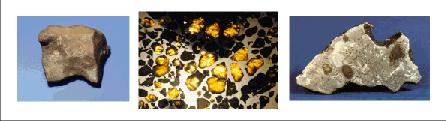
Iron meteorites contain genuinely reduced metal, sufficiently well refined by nature that the cut and polished face of an iron is highly reflecting. It has been suggested that the existence of these stones gave early man the notion of refining metal from ores. There are records of iron meteorites being used as ploughs by farmers--after appropriate treatment by a blacksmith.
The reduced metal in iron meteorites is actually one of two alloys, of iron and nickel. These alloys are usually considered among the minerals classified as native elements (Lecture 14). The minerals differ in their nickel content, with one of the alloys containing as much as 65% nickel, and physical properties. These differences make it possible to tell something about the freezing history of the meteorites from the intergrowth of crystals of the two minerals.
On crystallization, a mixture of the two nickel-iron alloys
will grow together in a distinct patterns that can be revealed
by polishing the surface of the meteorite, and then etching it
with acid. There results a crisscrossed pattern known for
the inventor of the technique, Widmanstatten. Measurements
on this pattern reveal the cooling history of the meteorites.
It has been found that some of them cooled very slowly, at
rates of only a few degrees in a million years. This is surely
a clue to the manner in which these materials formed. How
and why might such cooling occur? We shall address this below.
Stony meteorites are of two types. Traditionally, a division into one category or the other was made by the presence or absence of small inclusions called chondrules, shown at the right. Most chondrules igneous in nature, but we are not sure how the melting took place. One theory is that it did so in the solar nebula, because of electrical discharges, or lightening. These melted small bits of material with rocky composition, making droplets which froze to form the rounded chondrules.
The most common form of chondrule is rounded, and we know that it is igneous in nature from geological thin sections. Other inclusions, sometimes also called chondrules, are irregular in shape, and may never have been melted. In some cases, it seems that rare kinds of chondrules may be solids that formed before the birth of the solar nebula, and were never mixed with it in a vapor phase. We will generally use the terms ``fragments'' or ``inclusions'' rather than chondrules for the non-igneous components of stony meteorites.
The word ``chondrule'' comes from the Greek root meaning cartilage--it isn't a very helpful mnemonic. Meteorites that contain chondrules are called chondrites. Those without chondrules (with one important exception) are called achondrites. Most of the achondrites are mafic or ultramafic (no quartz or feldspar) igneous rocks. We are convinced that some achondrites came from the Moon and from Mars. Others show almost the identical reflection spectrum of the minor planet Vesta.
Stony irons are, as one might anticipate, a combination of the two kinds of meteorite. The cut face of a stony iron might reveal a polished metal framework, with green crystals of olivine in little cells where the metal was missing.
Most of the meteorites in museums are irons. This is because they are the most easily recognized as something distinct from terrestrial rocks. The majority of these irons are `finds.' Most `falls' are chondrites. We may conclude that the majority of the meteoroids are rocky rather than metallic in nature. More than 80% of the falls are chondrites.
The falls of several meteorites have been recorded photographically, so that their orbits could be determined. These are shown schematically in Figure 35-2.
The figure shows orbits of Mercury and Venus (inner circles), Earth, Mars, and Jupiter. These are shown in blue. The green ellipses are meteoroid orbits corresponding to five meteorites. The most recent of these, Taglish Lake fell in January 2000 in British Columbia. The figure shows close spacial association of these objects with the asteroids, whose orbits are concentrated in the region between Mars and Jupiter.
Meteoriticists had long discussed the possibility that meteorites were debris from the failed planet or planets that were once in the asteroid belt. Such a hypothesis would account for the existence of igneous material, and core-mantle differentiation in a putative parent body would account for the iron meteorites.
There is one problem with the postulate of complicated igneous activity on asteroids. They are small bodies, and could lose their heat quite rapidly. Consequently, it is unclear that they would have retained enough heat to form cores, and igneous melts. What source or processes might have supplied the required heat?
Among the nuclides that have been investigated in physics laboratories there are a number that have half-lives much shorter than the heat sources we discussed in connection with the earth and Jovian planets. Let us explore why such radioactivities are important for the asteroids.
 Long     Half-life       Short     Half-life

 K-40      1.28E09        Al-26     7.3E05
 Th-232    1.4 E10        Ca-41     1.03E5
 U-238     4.47E09        Fe-60     1.5E06
 U-235     7.04E08        Pu-244    8.0E07
The sources we have discussed--uranium, thorium, and potassium--have long half-lives and supply heat very slowly. Now if a body is to heat up, it is necessary that the energy not leave the body at a rate comparable to that with which it is supplied. How fast does a body cool?
Let us assume that any energy flux
(energy per unit area per sec) that
reaches the surface will be radiated away. In other words, we assume
the surface temperature will rise until it reaches a value such
that T4 equals the energy flux
from below (joules meter-2sec-1 or
ergs cm-2sec-1). Then the rate of cooling
of a body will depend on how fast the transport mechanisms can
carry the energy to the surface. This depends on the nature
of the transport mechanisms, but for purposes of argument, we
assume the relevant mechanism is conduction.
If we have two bodies with equal conductivities, it is possible to show that the cooling times will depend on the squares of their characteristic dimension. This means that a spherical body with radius R would cool 4 times faster than a similar body with radius 2R.
Detailed calculations show that small bodies would cool too quickly for the long-lived radioactivities to heat them to the point where core formation could occur. We can make up a little table based on the cooling time for the Moon.
characteristic length     typical body      cooling time (years)
or radius (km)                             E9 means x ten to 9th

2000                      Moon                1. E9
 200                      large asteroid      1. E7
  20                      small moon          1. E5
We see from Tables 34-1 and 34-2 that the long-lived radioactivities are capable of reheating the Moon--and causing the impact basins to flood. This takes place on a time scale of the order of half a billion years. Even for asteroids, the cooling times (1 x 10⁷ years) are 3 to 4 orders of magnitude shorter than the half-lives of 232Th, 238U, and 40K. Perhaps 235U could be relevant. For smaller bodies, the shorter half-life isotopes are clearly important as heat sources.
We shall see in the next lecture that there is good evidence that these short-lived isotopes were present in the early history of the solar system.
What about the collisions themselves as heat sources? Surely this is relevant, but most discussions have not taken them into account. Perhaps good quantitative estimates have not yet been made.
We conclude that meteorites come from chemically differentiated bodies primarily in the asteroid belt.
Among the chondritic meteorites there is a class known as the carbonaceous chondrites (CC's). These meteorites consist of chondrules and a great variety of mineral fragments imbedded in a matrix that is rich in carbonaceous material. The carbonaceous material is heterogeneous, and includes soot and organic polymers. Considerable interest focused on the presence of amino acids in CC's, but there is little basis to conclude that these simple organic compounds are the product of life.
Astronomers have known for most of the present century that the elemental composition of chondrites mimicked that of the sun for non-volatile elements. From about 1950 through perhaps 1980 there was a competition among meteoriticists to find which among the meteorites most closely resembled the solar composition. This ``race for the Holy Grail'' will be described in the next lecture.
Eventually, the Swiss-American cosmochemist Edward Anders won the prize with his advocacy of meteorites known as Type I carbonaceous chondrites. We will call these special meteorites the CI's, for short. These meteorites are an exception to the rule that chondrites contain chondrules. Indeed, they appear to be quite similar in their entire composition to the carbonaceous background matrix of other carbonaceous chondrites. Roughly speaking, if you took the chondrules and some hard mineral fragments from a carbonaceous chondrite, and compressed the remains into a rock, you would have a Type I carbonaceous chondrite.
It has been important to establish the Holy Grail (SAD) because of the role it plays in theories of the origin of the nuclides. Since the late 1950's it has become clear that the majority of the chemical elements and their isotopes (nuclides) were manufactured in the interiors of stars. These processes have left their signature in the abundance patterns in the SAD. Just as the geochemist can read the history of rocky materials from their mineralogy, the astrophysicist can read the nuclear history of matter from its abundance patterns. We shall have more to say about this in the ensuing lectures.
The Age of Enlightenment had a blind spot for meteorites. In the nineteenth century their extraterrestrial nature was again recognized, and productive research could proceed. The three broad classes of meteorites, stones, irons, and stony irons correspond roughly to planetary mantles, iron cores, and core-mantle boundaries. Meteorites that have been seen to fall are called falls, while those subsequently discovered are called finds. Most finds are irons, because they are easy to recognize. Most falls are chondrites. The achondrites are mostly igneous stony meteorites. A number have been identified with a planet, satellite, or asteroid.
Orbits of several meteorites indicate an origin in the asteroid belt. We believe they came from differentiated minor planets that were broken by collisions. Short-lived radioactive isotopes can provide the necessary heating for core-mantle differentiation.
The carbonaceous chondrites, and particularly the Type I Carbonaceous Chondrites (CI's) provide the best guide to the SAD and the nuclear history of matter.
The meaning of the term SAD (standard abundance distribution) changes subtly from one usage to the next. This is a general problem with language, and it is why dictionaries typically give more than one meaning for individual entries. Let us examine some of the various meanings of this term. The SAD may mean:
Meaning (1) refers to a specific set of numbers assembled by some individual or group of people. These workers attempt to find the best estimates of the solar composition--meaning (2). The problem is that solar abundances can not be determined as accurately as those in meteorites. Experience has shown that as the solar determinations improve, for most elements the relative abundances in the sun and the Type I carbonaceous chondrites (CI's) agree with one another.
The elements that fail to agree in the sun and the CI's are what we have called the supervolatiles: hydrogen, helium and the noble gases, carbon, oxygen, and nitrogen. With the exception of these few elements, there is no basis to say that the relative solar and CI abundances differ from one another. This situation could change, as the accuracy of solar abundances improves, but for the present, we have the rather bizarre situation that certain special rocks (meteorites) tell us what the sun is made of better than the sun itself!
We assume that because most of the mass of the solar system is tied up in the sun, the sun should be the most representative object of the primordial cloud from which sun and its planets originated. Thus we have definition (2) for the SAD, and we see that we are really using the sun as a means to get at definition (3)---astronomers want a representative set of abundances for our location in the Galaxy. It is possible that the sun is special in some way, and that its abundances are not ``typical.'' For example, it is generally known that the abundance of oxygen generally measured in hot interstellar gas is lower than assumed for the sun.
Oxygen is a super volatile, so that the value that appears in our table of the SAD does not come from the CI meteorites. For oxygen and some other super volatiles, it comes from spectroscopic determinations of the solar composition. Generally, these are much less accurate than meteoritic determinations, but for the supervolatiles, we must use them. From the best information we have, it appears that oxygen in the sun is rather higher than the average in the Galaxy near the sun. So if we used definition (4) for the SAD, we would have a lower oxygen abundance than for definition (2) (and by default, definition (1)).
Qualitative chemical analyses of the sun and stars date from the early use of the spectroscope more than a century ago. In qualitative analysis, one determines the presence of substances, but not how much is present. When we measure how much, we are doing quantitative analysis. Quantitative analysis of the sun and stars dates from roughly the 1930's, and even in those times it was known that the relative abundances of many elements in the sun and meteorites were similar.
It is interesting that the theory of stellar spectra had finally progressed to the point where it was possible to say that the composition of most stars were remarkably similar. Now the spectra of stars are not similar. They look very different from one another.
Stars with the surface temperature of the sun are full of lines of neutral iron, while the spectra of the bright stars Sirius and Vega are dominated by strong lines due to hydrogen. In the first decades of the 20th century, astronomers thought the sun was made mostly of iron, and Sirius and Vega were mostly hydrogen. In the 1930's it became clear that the huge difference in the spectra of the sun and these two bright stars was caused largely by their different temperatures, and not by their composition.
It was a triumph of the theory of stellar atmospheres to be able to explain the diversity of stellar spectra in terms of physical conditions. Two basic principles were involved--the excitation and ionization of atoms. The average energy per particle--(3/2)kT--is not enough to excite hydrogen to the levels that give rise to the strong lines in Sirius and Vega. On the other hand, by the time the temperature has reached that in the atmospheres of Sirius and Vega, most of the neutral iron has been ionized away.
There were still a few stars whose spectra clearly indicated very different chemical compositions from the sun. However, these objects were apparently set aside in the minds of astronomers and knowledgeable geochemists. The notion of a universal abundance distribution began to appear in the scientific literature. As early as 1930, the term ``cosmic'' was used to describe what was thought to be the universal abundance pattern. Interestingly, the coiners of the term were analytical chemists whose specialty was meteoritics.
If we assume that the abundances of the chemical elements are the same everywhere in the universe, it is natural to seek one event where they were all made. This led the incomparable George Gamow and his coworkers to the early theory of the big bang. They sought some way in which all of the chemical elements could be created in the initial explosion that gave birth to our universe. Their work, which was done in the 1940's and 1950's had only limited success. They could never make elements heavier than helium! However, they predicted the cosmic background radiation long before its discovery. In addition, we now accept a nearly universal helium abundance, and that it emerged from the big bang.
Nucleosynthesis is the name given to the processes that made atomic nuclei. After stellar nucleosynthesis (Lecture 7) became accepted, is was clear that abundances in stars must vary. These variations are not large for the majority of stars, but important and occasionally quite large variations do occur. For this reason it is no longer appropriate to speak of a `cosmic' abundance pattern. Nevertheless, the four meanings of SAD given above are all useful concepts. The French nuclear astrophysicist Jean Audoze and the American astronomer Beatrice Tinlsey suggested use of the phrase `standard abundance distribution' (SAD) as a replacement for the anachronistic `cosmic abundances,' which is still occasionally used.
Even though the SAD may not be ``cosmic,'' it is still of keen interest, and the question naturally arose of how best to get at it. In principle, spectroscopic analyses of the sun's atmosphere would be the best way to proceed. Unfortunately, these determinations were notoriously inaccurate, and they gave almost no information at all on isotopic abundances. Meteorites thus persisted as being the best overall guide to the SAD, but there are many and varied kinds of meteorites. Which ones would be the best guide to the SAD? An American cosmochemist compared this quest with that for the Holy Grail.
Possibly since the heyday of ``cosmic abundances'' we have assumed that the abundance pattern we seek should reflect nuclear rather than chemical properties. That's because the nuclei had to be made by nuclear processes, and the results should reflect nuclear rather than chemical properties.
We have seen a plot of the SAD in which relative abundances vs. the atomic number Z are displayed. Nuclear astrophysicists have found a similar plot somewhat more informative. We show that here. Abundances are plotted vs. the mass number A rather than Z.
We will not go deeply into the theory of nucleosynthesis that accounts for the details of this plot, but we shall outline the salient points. They are generally accounted for in terms of nuclear rather than chemical properties. Generally speaking, those nuclides that are more stable are the more abundant.
We understand why the bumps occur on the abundance curve for heavy nuclei. It is closely related to the stability of nuclei. This stability derives from shell closing, that is similar to the closing of electronic shells or subshells. However, the number of nucleons that belong to closed shells is different from that of atomic shells because the nuclear forces are different. For a long time, physicists did not know why nuclei with certain special numbers of nucleons were very stable. One famous physicist said it was ``magic,'' and the term stuck. Thus, the bumps on the abundance curve are due to nuclear magic numbers.
Let us briefly note what we mean by a nonnuclear abundance pattern. A good example would be the earth's crustal abundances (Figure 19-2), with their depletions of the siderophiles, and severe depletions of the noble gases. These patterns exist because of chemical properties of elements. In this section we have mostly discussed abundance patterns that exist because of the properties of atomic nuclei.
As our knowledge of the structure of the atomic nucleus improved, it could be integrated into the search for the most representative meteorites. The search for these objects, improvements in our estimates of the SAD (at that time, the cosmic abundances), and our knowledge of nuclear structure and systematics went on simultaneously.
In the late 1960's, the Swiss-American cosmochemist Edward Anders and his colleagues narrowed the search for the Holy Grail to the Type CI carbonaceous chondrites. The strongest piece of evidence in favor of these meteorites was their high volatile content. Remember that volatiles are defined as materials that remain in the vapor phase of a cooling gas. We will simplify the argument given by Anders and his colleagues in the following paragraph:
Suppose you had a box full of the primordial gas of the solar nebula, and you cooled it until all of the vapor had condensed as solid material. Surely, this would be the long sought cosmochemical Holy Grail. Any subsequent heating of this solid would drive off sequentially the most volatile materials. The greater the heating, the further the composition would depart from that of the primordial nebula.
The most volatile-rich meteorites known are the Type I carbonaceous chondrites (CI's). They lack the igneous materials, the chondrules, which have undergone heating and melting. This would drive off the volatiles components of the chondrules. The overall volatile content of these meteorites varies inversely with the igneous fraction. The CI's contain no chondrules. CM's do contain this igneous material, and the CV's have still more. Consequently, the latter types have fewer volatiles (See Figure 35-4).
We assume the CI's have lost the least of their original material, and therefore choose them as the best approximation to the primordial composition. Of course, even the CI's have lost their supervolatiles: hydrogen, helium, nitrogen, (most of their) carbon and the noble gases.
In Figure 35-4 we compare the volatilities of two carbonaceous meteorites, called CM's and CV's, with the CI's. Logarithms of ratios of elemental abundances are plotted on the lower part of the graph, with the scale to be read for the y axis on the left. All three meteorites have approximately the same abundances for Mg and Si. The abundance ratios are therefore unity, and its logarithm is zero. Volatile elements plot as negative numbers. For example, zinc (Zn) is about half as abundant in the CM's as the CI's. The ratio is therefore 1/2, and the logarithm -0.3. This is plotted on the solid line. The ratio is about 1/4 for the CV's divided by the CI's, so the logarithm of the ratio is about -0.6 (dashed).
The logarithm of the condensation temperature is plotted in the upper part of the diagram, with the scale on the upper right. High condensation temperatures fall high on the plot, and low ones, low. This curve was generated with the help of the thermodynamic properties of real materials--compounds rather than elements--likely to condense from the gas of the solar nebula.
First, we see that the theory and the meteorites tell the same story about volatility. It isn't perfect, but the correspondence is too close to be accidental. Also, we see that the CM's and CV's agree about what is volatile, and with a few exceptions The CM's have about half the volatile depletion of the CV's.
Arguments that the CI are the most volatile rich, and that they have not been heated would not be worth much in the absence of two conditions:
The figure shows the difference in the logarithms of solar photospheric and CI abundances. The points for elements are indicated by their chemical symbols. The x-axis is the condensation temperature--the same quantity that was plotted vertically in Figure 36-2. Most of the abundances differences are within 0.3 in the logarithm, which is a factor of two. However, a few elements Lu, W, and Tb have larger differences. In the case of the element Lu (lutetium), a recent study obtained a result that moved the point as indicated by the long arrow. There is still not perfect agreement, but it was improved.
Suppose the CI meteorites really are the best indication of composition of the original solar nebula. Then improved solar abundances will bring all of the points in a plot such as Figure 36-3 to cluster closely about the line where the difference is zero.
There is now little argument among astronomers and meteoriticists that the CI's are the best guide among cosmic materials to the composition of the primitive solar nebula. This is only true because we can't analyze the solar composition very accurately or thoroughly---we can't get isotopic abundances for most elements. If we could get this information from spectroscopic analyses, the CI's would be displaced by the sun itself.
The mystery of the CI's is that these rocky materials are clearly chemically evolved. The source of their volatilities is in many cases hydrated minerals such as those found late in the Bowen series--carbonates and sulfates with water of hydration. Geologists with a great deal of experience have said it is extremely difficult to imagine the materials of the CI's were not in contact with liquid water.
Meteorites presumably came from asteroids that broke up. Perhaps it is reasonable to think that liquid water might have been present on these asteroids. We now believe there might be a liquid water ocean beneath the surface of the Galilean satellite Europa. Why not such an ocean on some asteroid?
The general problem with this is that water is a great solvent. If water flows into a region, it will bring with it dissolved chemicals. Should it evaporate in that region, those chemicals would be left behind. While it is in a region, it will dissolve some of the chemicals originally there. If it were to then flow away, it would carry those chemicals out of the region. We see that along with the presence of water, there is the strong potential to alter the bulk chemistry of materials that come in contact with it.
The mystery of the CI's is that the great potential for chemical differentiation was not realized. Or perhaps it was realized, but so slightly that we have not yet been able to detect it.
The solar composition might be taken as the SAD by definition,
but we cannot determine it very accurately. Consequently
the quest has led to the Type I carbonaceous chondrites (CI's).
Apart from supervolatile elements, these meteorites match the
sun as closely as we can tell. Their abundance pattern
bears the imprint of the atomic nucleus as well as a variety
of processes of nucleosynthesis: hydrogen and helium
burning, silicon burning, the  -process,
and rapid (r) and slow (s) neutron addition processes.
-process,
and rapid (r) and slow (s) neutron addition processes.
The CI's are the most volatile rich of the meteorites, and do not contain igneous materials--they have not been heated to high temperatures. Even though they show abundant evidence of aqueous alteration, there is no evidence in their bulk abundances of nonnuclear abundance signature, e.g. a depletion of siderophiles.
It has been possible to measure the relative abundances of isotopes of chemical elements since the invention of the mass spectrograph by Aston in 1919. These isotopic abundances, unlike the elemental abundances, did not seem to vary from one sample of materials to another. It was known that radioactive decay would lead to small isotopic variations, for example, in lead isotopes. For stable elements variations were slow in coming. Aston himself, wrote in his 1924 book Isotopes
...the evolution of the elements must have been such as to lead to a proportionality of isotopes of the same element which was constant from the start, and since we know of no natural process of separation, has remained constant ever since. The isotopes of lead formed by radioactive disintegration are exceptional.
Gradually, small variations in isotopic abundances were detected, and measured. These variations were all of a special kind that could be attributed to what we have called mass- dependent fractionations. We have discussed some of these in Lecture 19. In chemical reactions, there is a tendency for the heavier isotopes to be more tightly bound. To take a very simple example, in a reaction of carbon and oxygen to form the diatomic molecule carbon dioxide, there would be a slight tendency for the molecule to contain a higher percentage of the heavier isotopes of carbon and oxygen than there were in the reacting gases:
Atomic Carbon (12C and 13C) + Atomic Oxygen(16O, 17O, and 18O)
---> Carbon Dioxide(12C16O, 12C17O, 12C18O, 13C16O, 13C17O, and 13C18O)
For a reaction of this kind, the carbon monoxide molecules would be richer--percentage wise--in the heavier isotopes, than the atomic reactants.
To use our old analogy, the potential well for molecules with heavier isotopes is a little deeper than the well for the lighter isotopes.
In Lecture 19, we also discussed the effects of small, mass- dependent fractionations in water, as a result of phase changes. There was the somewhat counterintuitive result that the polar ice was depleted in the heavier oxygen isotopes as well as 2H (deuterium). You might think the ice would be enriched in the heavier isotopes, because the ice is cold. But the ice is formed from snow that comes from evaporated water in the oceans near the ice caps. And the water molecules with lighter isotopes tend to evaporate a little faster.
These mass-dependent effects are usually quite small, but they can be measured with mass spectrographs.
Still, for many years, it was believed that apart from radioactive and mass dependent effects, the isotopic abundances of the elements was constant within the solar system. This constancy became dogma. In a 1965 review, Hans Suess, one of the truly great pioneers in the field of cosmic abundances wrote:
Among the very few assumptions which, in the opinion of the writer, can be considered well justified and firmly established, is the notion that the planetary objects, i.e. planets, their satellites, asteroids, meteorites, and other objects of our solar system , were formed from a well-mixed primordial nebula of chemically and isotopically uniform composition.
In the late 1960's the theory of stellar nucleosynthesis made it seem clear that there must be widespread variations in the isotopic composition of material in interstellar space. Nuclear processes act directly on nuclei, and in contrast to chemical reactions, were predicted to produce large isotopic variations in stars.
Chemical reactions usually produce small, mass-dependent, variations in isotopic compositions. Generally speaking, electrons govern chemistry, and the electronic structure is the same for isotopes of the same element. Thus, chemistry cannot easily account for isotopic variations.
We note that the term nuclear chemistry is often used to describe nuclear reactions. Nuclear reactions can be written in a manner analogous to chemical reactions (see examples following Table 37-1), although physicists have an alternate scheme. Analytical chemists who use methods of neutron activation, may call themselves nuclear chemists. We should be clear, however, that nuclear processes act selectively, and individually on isotopes, while ordinary chemical processes do not. Thus, stellar nucleosynthesis should have created a variety of isotopic abundance patterns.
Throughout the 1960's, workers sought evidence of isotopic variations in meteorites, but with little success. Then in the early 1970's, pandora's box finally opened.
The earliest isotopic abundance variations were found for the oxygen isotopes (Figure 22-1). In a few years enough measurements had been made of meteorites of various kinds that it became generally accepted that different locations in the solar system had characteristic oxygen isotopic patterns. We made the argument in Lecture 23 that the identity of the oxygen isotopes in the earth and Moon were a difficulty for the Big Whack hypothesis. The standard answer to this problem is to assume the "impactor" formed very near the earth's distance from the sun. It could then have had the same oxygen pattern as the earth and Moon.
By the end of the 1970's a wide variety of isotopic abundance variations had been found. Why had they not been noted earlier? Workers in this field point out that many of the early anomalies were found in the CV carbonaceous chondrite named Allende. The interesting point is that Allende was a large meteorite, that fell near a small Mexican town just south of the US border in 1969. Meteoriticists from California went south with pickup trucks, and soon had large samples with which to work.
Prior to Allende, the main sources of meteoritic material were museums, whose curators were reluctant to give away large samples, even to established workers. It also was fortunate that Allende was rich in the kinds of inclusions that yielded new and interesting isotopic results. These fragments are often called calcium-aluminum inclusions or CAI's because the predominant minerals were rich in these elements. Corundum, Al2O3, and anorthite CaAl2Si2O8, are typical of the minerals of the CAI's.

Figure 36-1 shows numerous rounded chondrules as well as white CAI's (lower left, and center right).
While it is true that Allende was available in relatively large supply, and at the right time, it is also true that analytical techniques were being refined so that many of the exciting modern results of meteorite research would have soon been obtained, even if Allende had not fallen.
Several different kinds of isotopic effects were found:
One of the earliest pieces of evidence for an extinct radionuclide came from an examination of the relative abundances of xenon isotopes on the earth. As we have already noted (see Figure 19-2), there isn't very much xenon in the earth. There is a tiny amount in the atmosphere, and a little that can be cooked out of rocks. But xenon was mostly left behind by the materials from which the earth was formed. The little that is now present was either captured from the solar wind, or brought in, adsorbed or accidentally enclosed in planetesimals bombarding and forming the earth.
Xenon is a rather heavy noble gas. It is located at the end of the fifth (or second, long) period that begins with rubidium. Like all noble gases, it has an even number of protons. We would expect those isotopes with even numbers of neutrons to be more abundant than those with odd. This is the effect that gives the sawtooth pattern on the plot of abundances vs. A, and it's generally true for neutrons just as it is for protons (Figure 35-3).
Figure 36-2 shows that the most abundant xenon isotope is actually 129Xe--not at all what we would expect. How might this be explained?
The most reasonable explanation for the anomalously high abundance of 129Xe is that it is the decay product of 129I, iodine-129. This is not the common isotope of iodine. That's 127I. Indeed, 127I comprises 100% of terrestrial iodine. There is no more 129I because it has a half-life of 1.6 x 10⁷ years! Whatever 129I there once was has long since decayed radioactively to 129Xe.
While 1.6 x 10⁷ years is too short a half-life for 129I to be present in the earth now, it could well have been present in the early solar system. At that time, it would have behaved chemically just as the stable isotope of iodine did. Suppose iodine were imprisoned in rocks that formed early in the history of the solar system. If it were early enough, both the stable 127I and the radioactive 129I would have been captured. It is then possible that these rocks today would contain a sizable excess of 129Xe.
Of course, if the rocks had been heated at some point during the 4.5 billion year history of the earth, the xenon could have been driven off. Even so, it could make a noticeable contribution to the net amount of the earth's xenon, since there isn't much to begin with.
In some very ingenious analytical work, cosmochemists have investigated xenon that they cooked out of meteorites. There isn't much gas in a stone, but with the marvelous analytical techniques available today, it is possible to analyze the little gas that comes off. These workers found excesses of 129Xe in the meteorites. But in addition, they were able to show that the excesses were higher in those stones that had more of the stable 127I. This is strong evidence that the 129Xe was captured in the stones as 129I.
We take it as evidence for the presence of the extinct radionuclide 129I in the early solar system.
We have mentioned 26Al as a possible source for melting and core formation among the small bodies of the asteroid belt (see Table 34-1). What is the evidence that this isotope was present in the early solar system?
The problem of establishing 26Al is a little more difficult than with 129I, because 26Al decays into 26Mg. While there is very little xenon in the earth, there a great deal of magnesium. There are three stable isotopes of magnesium, 24Mg (79%), 25Mg (10%) and 26Mg (11%). Even though 26Mg isn't the most abundant of the three isotopes, there is so much magnesium in the earth, there is still lots of the heavier isotope.
Figure 36 - 3: Isotopes of Mg, Al, and Si, showing the decay of the unstable 26Al to 26Mg. As in usual nuclide charts, the number of protons in the nuclei (Z) is plotted vertically, and the number of neutrons (N), horizontally. Stable nuclei are gray.
How would it be possible to demonstrate a tiny excess of 26Mg due to the decay of 26Al? The answer is to investigate a mineral that would only have trace amounts of magnesium. Then any little excess might have a chance to show up.
This figure shows the result of the analysis of a fragment of the famous Allende meteorite. Ratios of 26Mg to 24Mg and 27Al to 24Mg were measured in four minerals of the fragment. The two minerals on the lower left have relatively little aluminum, while the two that lie higher up are both anorthite (CaAl2Si2O8), which has lots of aluminum. What is also important is that the anorthite is a tightly bound crystal, with little room for magnesium. What little magnesium there is, distorts the crystals, and a relatively small amount is incorporated.
It is because so little magnesium is accommodated in the anorthite that the small amount of 26Mg that comes from the radioactive 26Al is detectible. The results shown in Figure 36 - 4 come from impressive experimental work done at the California Institute of Technology by Gerald Wasserburg and his colleagues. These workers developed ultrasensitive mass spectrographic techniques that have been adopted in laboratories around the world, including one in the Geology Department at the University of Michigan.
We are made of stardust. Most of the chemical elements were synthesized in stars. Stars formed out of the interstellar gas and began their lives converting hydrogen to helium, and helium to heavier nuclei. These stars eventually exploded, or in some cases, oozed part of their nuclear ashes back into the interstellar medium. The next generation of stars incorporated some of this material, and at the end of their lives, added their own contributions to the slowly accumulating stock of heavy elements. Astronomers often refer to the mass fraction of these heavy elements by the symbol `Z' (see Lecture 7).
The interstellar medium into which heavy elements are ejected roils with the blast waves of supernovae and high winds from massive hot stars. It is generally thought that these forces mix the gases rather thoroughly between star-forming epochs. Thus any gas cloud from which stars might form would be a mixture of compositions, from the most primordial, just hydrogen and helium, to the most highly enriched in Z.
The long failure to find isotopic abundance variations between meteorites and terrestrial materials is not without meaning. The interpretation given by Aston and Suess was that the solar system itself had been thoroughly mixed.
Now we are reasonably sure that grains of dust form in the atmospheres of cool stars. These dust grains should bear the signature of nuclear processes peculiar to the stars in which they formed. Workers expected to find some of these grains in meteorites, but for many years, they found nothing. Consequently, they postulated that the solar nebula itself had once been heated by its own gravitational collapse to such a high temperature that any residual solids would have been vaporized. The vapor would have been homogenized--mixed--by turbulent currents within the early solar system.
This scheme would--and does--account for the isotopic homogeneity of most of the solid material from the solar system that we have been able to analyze.
Some isotopically anomalous fragments have now been found. This means, first of all, that not all of the solids were vaporized when the solar system formed. Just what fraction of the mass of meteorites might have been unvaporized? No one knows for sure. Estimates vary from about 1% down to 0.01% (10-2 to 10-4). But it is a simplification to simply give an overall fraction for the unvaporized material. Current studies account for a variation in this fraction: the closer toward the center of the solar nebula, the lower the fraction of surviving solids. This, of course, is because it would be hot closer to the center--to the sun--and therefore more likely any grain would be vaporized.
The calcium-aluminum-rich inclusions--the CAI's--typical of the irregular fragments of the Allende meteorite were among the first materials to show isotopic variations from the standard. Even now, we are not really sure of the origin of these inclusions. Some think these fragments were ``mostly'' formed in the solar system from vapor, but that they contained small amounts of materials that never vaporized. This is in general agreement with our notions of truly presolar grains, truly unvaporized solids that formed prior to the beginning of the birth of the solar system.
It is interesting that the first inkling of such materials were found by the imaginative Edward Anders and his coworkers. This is the same Anders responsible for the recognition of the CI meteorites as the best source of SAD abundances.
Anders had been in pursuit of evidence for extinct radionuclides that might have been much heavier than uranium and thorium. After the theory of the atomic nucleus was worked out to the extent that the magic numbers were understood, physicists realized there might be certain superheavy nuclei with extra stability. According to predictions, these nuclei might have mass numbers near A = 298.
Few thought that these superheavy nuclei would be stable, or have half-lives of billions of years. But it was conceivable, based on the theory, that they might have half-lives of the order of 105 or 107 years. The superheavy nuclei would probably decay by fission. The fission fragments would initially be neutron rich, but they would beta decay and become stable, lighter nuclei. Some of the fission fragments might end up as heavy isotopes of xenon. Anders and his coworkers were looking for evidence of this.
Xenon is highly depleted in all meteorites, but there is more in carbonaceous meteorites than in most. One had to cook it out of the rocks, of course, by heating them, and then analyzing the gases with a chromatograph or mass spectrometer. But what kinds of material contained the strange xenon?
Anders eventually devised the technique which he colorfully described as ``burning down the haystack to find the needle.'' It turned out that if one dissolved most of the carbonaceous meteorites in a potent acid mixture, a few small grains remained. These were often only a micron (10-4 cm) in diameter, but they were found to be the source of the anomalous xenon.
These acid-resistant residues comprise what we now call the presolar grains. They are generally carbonaceous, though they are tough carbides, graphite, and diamonds rather than organic compounds. The diamonds are tiny, of the order of 20 Angstroms in diameter. Recall that 1 Angstrom is a typical atomic dimension. Note that 20 Angstroms is also 2 nanometers, and for this reason, the diamonds are often called ``nanodiamonds.'' Sadly, there are no multimineralic samples, so thus far, we cannot get ages for them.
Anders was never able to clearly demonstrate the presence of superheavy (A ca. 298) nuclei in the early solar system. Some of the anomalies he had looked at, especially in xenon, might be explained from the decay of 244Pu, Plutonium-244, which has a half-life of 8 x 10⁷ years. The 244Pu is quite interesting in its own right, and studies of other elements have opened an entirely new field of meteorite and astronomical research.
The presolar grains give us information about stellar nucleosynthesis that was never available before. We could study the spectra of the stars, of course, but generally we could not get any information on isotopic abundances. Spectra are generated by atomic electrons, and these are not very sensitive to differences among isotopes. Now, with material available in laboratories, a trove of new information is available on isotopic abundances beyond the solar system.
The main advantage the presolar grains have over ordinary meteorites is that they are not so severely mixed. In the case of the solar system, we think the original gas was thoroughly stirred, both before the system formed, and during formation.
We cannot be sure of the history of the presolar grains, but it is highly probable that some were formed in the atmospheres of stars that were in the process of cooking heavy elements. If these solids then made their way to the earth, they would carry the chemical signature of nuclear processing in an individual star. While we can't see which star the grain came from, we can calculate the kinds of abundances that might be created in certain kinds of stars. When these calculations have been compared with the analyses of some presolar grains, the agreement has been excellent. In particular, we get confirmation of the processes that make some of the heavy elements indicated on Figure 35-3.
The presolar grains have contributed to our knowledge of nucleosynthesis in exploding stars and red giants. This exciting field is still in its infancy.
Long after the invention of the mass spectrograph, and our ability to measure isotopic abundances, it was thought the solar system was isotopically homogeneous. This conclusion excludes mass-dependent fractionations and radioactive effects that were well understood. The homogeneity led to the conclusion that the solar nebula had been thoroughly vaporized and mixed. Oxygen isotopic anomalies were measured in the CAI's of Allende and other meteorites, and led to the conclusion different regions of the solar nebula had different oxygen isotopic abundance signatures. The CAI's provided evidence for extinct radioactivities, e.g. 26Al, 129I, and 244Pu. No conclusive evidence was found for superheavy nuclides, but the search for them led to the discovery of presolar grains. These bear the signature of nuclear processing that is dominated by a single star. Solar system isotopes result from a well mixed Galactic gas, and have contributions from a wide spectrum of nucleosynthetic processes.
It is quite reasonable to describe the sun as a typical star. Stellar masses are not hugely different from the sun's. The lowest mass stars are about a tenth of the sun's mass, while the most massive stars are less than 100 solar masses.
The energy output of stars depends on the mass raised to a power between 3 and perhaps 5.5. This means that massive stars pour out energy at such prodigious rates that their nuclear fuel may be exhausted in a million years. The output of energy from a star influences the kinds of planets that can form near them, as we have seen in Lecture 29. The surface temperature of a planet is rather closely related both to its distance from a star, and the energy output from that star.
Astronomers have a reasonable idea of the distribution of stellar masses. This distribution would enable one to calculate the fraction of the total number of stars that have masses within some limits of the solar mass.
At one time it was fairly standard to think that life was most likely to arise on a planet near a star very similar to the sun. The argument was based on one data point, the earth! We know that there are planets about the sun, and that there is life on one of them. The searches for extraterrestrial planets have concentrated on stars similar to the sun.
In the following lectures, we shall point out rather compelling arguments that the essential condition for life is the existence of liquid water. These conditions might arise on any planet for which the energy balance, inflow and outflow, allowed temperatures between 0 and 100o Centigrade.
Therefore, we will not complicate our speculations by restricting them to solar-like stars. We may consider the entire gamut of some 1011 stars of the Milky Way Galaxy. If we extend our speculations to the universe itself, we need an idea of the number of such galaxies it may contain. No one knows this number with any certainty. A figure that is not unreasonable, is 1011, the same number as for stars in our Galaxy.
With all of these stars, it might seem compelling that our earth is not the only one with life.
If life arose spontaneously on the earth, it surely did not do so in a day, a year, or even 100 years. Classical experiments in biology have ruled this out, as we shall see in Lecture 40. Therefore, if most stars lived for only 100 years, it would be reasonable to rule them out as sites for planets that could support life.
Estimates of when the earliest life forms arose on the earth vary. For purposes of the present discussion, we shall assume the earliest cellular life forms appeared on earth some 500 million (0.5 billion) years after its birth.
We considered the lifetime of the sun briefly in Lecture 6. We now take up the topic for stars in general. Stellar lifetimes may be simplified into a rate equation. The rate of energy output multiplied by the lifetime must equal the amount of available energy. Stars shine because they convert some of their mass to energy by Einstein's famous E = mc2. Consider that
| Stellar Mass (Sun =1) | Stellar Lifetime (years) |
|---|---|
| 25 | 2 x 10⁶ |
| 10 | 1.9 x 10⁷ |
| 5 | 1.0 x 10⁸ |
| 3 | 3.3 x 10⁸ |
| 1 | 8.3 x 10⁹ |
| 0.6 | 6.9 x 10¹⁰ |
Stars that are burning hydrogen into helium are said to be on the main sequence. This is where stars spend about 90% of their lifetimes. There is a natural division in the structure of main sequence stars between one and two solar masses. The more massive stars are said to be on the upper main sequence, and the less massive, on the lower main sequence. There are two basic schemes by which hydrogen is burned to helium. In upper main sequence stars the primary mechanism is called the CNO-cycle. The most important reactions were first clarified by the Nobel Laureate Hans Bethe. The following reactions are called the Bethe cycle.
A 12C nucleus collides with a proton, creating an excited
13N nucleus, which jumps to the ground level by emitting a
-ray.
This 13N is unstable. It has too many protons.
Consequently, the nucleus relaxes by emitting a positive electron
and a neutrino in a form of
 -decay (Lecture 13). The
13C formed in this way absorbs another proton to give
14N, and so on. In the last step of the cycle, a helium
nucleus is released. The net result of Bethe's cycle is to
make helium out of four protons. The energy difference corresponding
to the mass of four protons and a helium nucleus can power a star.
-decay (Lecture 13). The
13C formed in this way absorbs another proton to give
14N, and so on. In the last step of the cycle, a helium
nucleus is released. The net result of Bethe's cycle is to
make helium out of four protons. The energy difference corresponding
to the mass of four protons and a helium nucleus can power a star.
Deep in stellar interiors, where these reactions take place, most electrons have been stripped by the high pressures and temperatures, so the nuclei collide like billiard balls. However, the nuclei are all positively charged, and repel one another. That repulsion must be overcome by having the nuclei move fast enough, and for this the temperature must be high.
Interestingly, the temperature at the center of the sun is not quite high enough for it to derive most of its energy from the Bethe cycle. Instead, it comes from the simple combination of protons in a fusion reaction. Essentially, the reactions are these:
Two protons combine to form a deuterium (or heavy hydrogen) nucleus.
The deuteron adds a proton to become an isotope of helium, with
two protons but only one neutron.
The 3He nucleus is formed in
an excited state, and it drops to the ground level with the emission
of a -ray.
Finally, two of the 3He nuclei combine to give
a 4He nucleus and two protons.
This scheme is called the pp-chain.
The net result of this process is essentially the same as that of the Bethe cycle, four hydrogen nuclei are converted to one helium nucleus, with the production of energy (and the emission of neutrinos). The positrons that are emitted, are quickly annihilated when they come in contact with ordinary electrons, and the result supplies heat to the solar interior. The neutrinos, however, escape from the sun completely, carrying their energy with them. These neutrinos have been detected at the earth, though there have been fewer detections than were expected.
We call the relative number of stars in different mass ranges the stellar mass spectrum.
It is fairly safe to say that most of the stars that are formed have masses of 3 times the solar mass or less (!!). Therefore, if life were to form on a planet near most stars, it would have a time of the order of 3 x 10⁸ or more do so. Slightly more than half of all of the stars formed have the solar mass, and for these objects, the available time stretches into the billions of years.
We see that while a few stars live only a short a time there is ample time for life to develop on the majority of them.
While stars spend most of their lifetimes on the main sequence, they eventually burn their allotment of hydrogen, and pass through a series of stages. The stars leave the main sequence, and become both cooler and larger. They become red giants. The envelopes of the red giants may swell to enclose any nearby planets, raising their surface temperatures to thousands of degrees Kelvin.
In the final stages of stellar evolution, stars either explode or become ``compact objects.'' By the latter, we mean white dwarfs, neutron stars, or black holes. Pulsars are thought to be the neutron-star remnanents of stellar explosions. Some stellar explosions may leave no remnanents.
The ultimate fate of planets engulfed by expanding stellar envelopes depends on many factors. Jovian planets would soon lose their complements of hydrogen and helium. Rocky or metal-dominated planets might survive the high temperatures longer. They would continue to orbit the center of mass of the swollen star, and the drag of the material would cause the planet to spiral toward the star's interior where it would eventually be vaporized.
It is interesting that the first planetary masses were found near pulsars, which are the remnants of exploding stars, or supernovae. It would be surprising if planetary objects survived the evolutionary phases of exploding stars. Some think these planets formed somehow after the explosions.
There are many double stars where one of the two objects is too faint to be easily detected. The binarity of these stars was discovered by noting irregularity of the path of the observable star. There are two basic ways this irregularity has been discovered: astrometrically, and spectroscopically.
Astrometry is the name given to the branch of astronomy that deals with various aspects of the positions of objects, stars planets (or asteroids!!). The root word "metric" arises because these positions are measured, and since the days of the telescope, measurements were made with a good deal of precision. Traditionally, the measurements were made of the positions of stars with respect to one another. Initially the measurements were made visually, using cross wires in the eyepiece of a telescope. Eventually, the separations of images on a photographic plate were measured. These astrometric measurements could be converted into angles-- the angular separation of one object from another.
Nearby stars seem to move slowly through the field of more distant stars. If they are close enough to the sun, their motion will also show a wobble, because they are viewed from different points in the earth's orbit. This wobble is used to determine the star's parallax.
In the case of binary stars, where both components are visible, there is also a motion due to the orbits of the stars about one another. Astronomers began to measure such relative motion early in the 19th century. By mid-century a curious phenomenon had been discovered. A few well observed stars, such as Sirius and Procyon seemed to show orbital motion about unseen companions. Eventually, these studies led to the amazing discovery of white dwarf stars, objects with the mass of the sun, but the size of the earth!
We must leave the fascinating study of white dwarfs to Astronomy 102/112 and web surveys, and turn briefly to a topic caught the attention of the press as well as professional astronomer's from time to time.
The star with the highest known motion across the sky was discovered by the American astronomer E. E. Barnard, and is known as Barnard's star. It is a faint, red dwarf, is among the half-dozen stars nearest the sun. Because of its motion, and its proximity, it was closely studied by astrometric techniques.
In 1963, the Dutch-American astometrist Peter van de Kamp announced that he had discovered a companion to Barnard's star. The announcement was received with some skepticism, but also with keen interest as van de Kamp was an acknowledged authority in his field. For at least a decade thereafter, van de Kamp would present updated versions of his results at astronomical meetings and in various publications. In 1975 he summarized the results of two decades of work, including more than a thousand night's observations and countless measurements: There were two companions to Barnard's star. One companion was certain, and had a mass about equal to Jupiter's. The second companion was less certain, but might have about half a Jovian mass.
Peter van de Kamp died a few years ago, still believing in the reality of his companions to Barnard's star. He was not the only one. Astronomers at the University of British Columbia published measurements that claimed three or more companions. Nevertheless, more recent work, including some based on observations with the Hubble Space Telescope have failed to confirm the presence of any companion to Barnard's star.
There are many cases in science like that of the companions to Barnard's star. An experienced, competent researcher announces a result that remains unconfirmed by others. Those quick to judge are often severe in their criticism: The scientist was not careful, or was too influenced by desire for a sensational discovery. But it is often the case that the scientific results lay within a domain of uncertainty where experts may legitimately differ. There should be no particular stigma about being wrong in such circumstances, provided only that one acknowledges the overall uncertainty.
Recent astrometric work on a famous red dwarf that is not unlike Barnard's star appears promising as the first detection by this method. The star is number 21185 of a catalogue published by Lalande in 1801. The new work, unlike that of van de Kamp, appears to be generally accepted. Perhaps this is because the discoverer, George Gatewood of Allegheny Observatory, is the same person who discredited the planets of Barnard's Star.
While unseen companions were first discovered by astrometric measurements, many more cases are known from spectroscopic studies. One observes the radial velocity of a star with the help of a spectroscope, and use of the Doppler effect. In general, this velocity will oscillate because of the earth's orbital motion. It's rotational motion can also be of importance. However, these effects can be removed from the measurements, and the star's radial velocity reduced to what it would be if it were observed from the sun. It is usually understood that these effects have been removed when a star's radial velocity is given.
A single star should thus have a constant radial velocity, A double star would show a radial velocity that varied periodically, as the two stars orbited one another. The only exception to this would be if the orbit of the pair were exactly perpendicular to the line of sight, so there would be no component of motion in this direction.
Generally, spectroscopic binaries are close enough together in angle that only one object is seen. The stellar image appears single in the telescope, and the only way we might know the star is double is from the spectrum. We shall assume the spectrum consists of absorption lines superimposed on a continuum, as this is the situation in the majority of cases. If the two stars are equally bright--intrinsically--then absorption lines from both stars will appear in the spectrum. These lines will move back and forth across one another, since one component of the system must be moving away if the other is approaching. Astronomers call such a system a double-lined spectroscopic binary.
More often than not, absorption lines from only one of the two stars are seen. This is the situation for the single- lined spectroscopic binary, and it is the case of most relevance for extrasolar planets. For this case, the ``unseen star'' is presumably not a star at all, but a planet.
Stars are a lot more massive than planets. The effect, even of
an unseen star is likely to be much greater on its companion than
a planet.
Suppose the sun and
Jupiter were the only objects in the solar system. Jupiter revolves
once about the sun in 11.86 years. For simplicity, take the orbit
as circular, and let us use 1000 as the mass ratio. This means that
in 11.86 years, the sun would revolve about the barycenter (center of
mass) of the system, which would be 0.001 of Jupiter's distance
from the sun. This is 5.203 x 10⁻³ AU, or
7.75 x 10⁵ This is about 13 meters per second,
a far cry from the radial velocities measured for
typical binary stars, which are several tens of km/sec.
Until fairly recently, stellar radial velocities were rarely measured
with an accuracy of even 1 km/sec. It would have been quite out of the
question to measure one to 0.01 km/sec.
This has changed in the last decade or two, largely as a result of
techniques that allow the entire stellar spectrum to be measured
automatically, relative to some standard.
Numerous web sites are now devoted to
this exciting new area.
Geoffrey Marcy and Paul Butler, of San Francisco State
University have been among the leaders in this field.
Their table of planet candidates lists 17 possibilities as of
April 1999.
One clear result of the recent surveys is that the newly found
systems generally do not resemble our solar system, and some can
be very different indeed. It should not be surprising that most
of the newly found planets are massive. The larger the planet,
the greater the influence on the radial velocity of it's parent
star. So most of the recent objects have Jovian or larger masses.
Current techniques are only beginning to approach the accuracy
necessary to find a planet with the mass of the earth. A
summary of 10 of these systems is shown below.
In this plot, the positions of the new planets relative to their
central stars is plotted on the x-axis. This can also be related to
the flux of energy from that star, which is given along the top of
the graph. The y-axis gives a lower limit to the masses of the planets.
Units are the Jovian mass. Note that Jupiter and Saturn are shown.
The stripe in the center of the diagram is calculated so that the
surface temperatures of the planets would be between 0 and 100C, or
liquid water temperatures.
The least massive planet in the figure is about half a
jovian mass--pretty massive! This is not difficult to understand
as a selection
effect: the more massive the planet, the easier it is to
detect.
It is also true that a planet closer to its parent star is
easier to detect than one further out. This is readily seen from
Equation (1) above.
Even though selection effects must have been very important
in these early discoveries of extrasolar system planets, they
are the only systems we know of, apart from our own. Astronomers
have begun to wonder if the general scenarios we have developed
to describe our own system are realistic. For example, in our
scheme, terrestrial planets formed in the inner solar system
because it was too hot for much other than metal and rock to
be in the solid phase.
If this picture were generally true, how did the massive
jovian planets illustrated in Figure 37-1 form?
Perhaps the answer is related to another property of some of
the newly discovered objects, their eccentricities. A few of
the new planets have eccentricities of the order of 0.4.
Their regular orbital paths thus take them toward and away
from their parent stars by substantial fractions of their
semimajor axes.
In the solar system, Pluto has the highest eccentricity,
0.24, mercury the next, 0.21, and all of the others are less than
0.1. In many-body systems, eccentric orbits are a sign of
instability, or change. Thus it is possible that the new planets
acquired their high eccentricities from interactions with other
unseen bodies. These might have caused the semimajor axes
of the planets to change with time--in the present cases,
decreasing.
More elaborate evolutionary schemes have been discussed
that might account for the structure of the newly discovered
planets. We cannot detail them here. This is a new and exciting
area, and we will hear much more about it in the future.
Stellar luminosities vary enormously, but the masses are
generally within 0.1 and about 50 solar masses. The most
massive stars live only a few million years, but at least half
of the stars have masses of a solar mass or less, and these
objects live for some 8.3 x 10⁹ years.
It would seem
that there is enough time, perhaps 0.5 billion years,
for life to have originated on a
good fraction of the stars in our Galaxy and universe.
Stars spend most of their lifetimes on the main sequence,
burning hydrogen to helium by the CNO cycle or pp-chain.
In the later stages of evolution, stars swell up and/or
explode, thus creating life-hostile environments.
Unseen planets may be discovered near stars either
by astrometric measurements or from their radial velocities.
The latter technique has born much fruit recently, although
the planets that have been found are generally rather
large, and close to their parent stars.
To nineteenth century geologists, the earth seemed timeless.
They had managed to mostly discredit notions that
the earth was a few thousand years old, which stemmed from
religious beliefs rather than science.
For most of their century, the principle of uniformatarianism
meant that there was no beginning or end to the earth.
Toward the end of the century, they were attacked from an
unexpected source.
The distinguished British physicist Lord Kelvin estimated
ages of the sun and the earth in the general range of a few
tens to a few hundreds of millions of years. One can easily
get an age of this order from the sun, by dividing
it's supply of gravitational energy by
its current
rate of energy output (3.96E33 erg/sec):
t(sec) = [(6.67E-8 erg cm/gm2 x
(2 E33 gm)2/6.9E10(cm)]/3.96E33 erg/sec = 9.8E14sec
In years, this is about 3 x 10⁷ or 30 million
years. Of course, this figure would give the age of the sun
if its energy were purely gravitational, and if it had been
radiating at its present rate.
Let us see how rapidly the sun would consume its mass if
it were a standard chemical source, such as crude oil. For
simplicity, we use a density of 1 gm/cm3,
although crude oil can be higher.
One barrel (bbl) of crude is 159 liters, or
1.59 x 105 cm3. If we assume unit density,
we get 1.59 x 10⁵ gm/bbl. Therefore, the sun's mass
is the equivalent of 2 x 1033gm/1.59 x 105gm/bbl
or 1.26 x 1028 bbl. Now 1 bbl of crude oil is about
5.8 x 10⁶ BTU/bbl or using 1.055 x 10¹⁰ erg/BTU,
we get 6.1 x 10¹⁶ ergs/bbl. So the total energy in
one sun's mass worth of oil turns out to be
1.26 x 1028 bbl x 6.1 x 1016 ergs/bbl
or 7.6 x 1044 ergs.
At a luminosity of 3.96 x 1033 erg/sec, this energy
would be expended in only 1.9 x 10¹¹ sec, or
about 6000 years. Maybe the good Bishop Ussher was right!
Seriously, we see that chemical energy is entirely inadequate
to supply the sun. This was readily calculated by Lord Kelvin,
who fixed on the only other source of energy known to him,
gravity.
Kelvin wasn't sure of the internal structure of the sun. This
means he wasn't sure of the little factor Geologists were quite unhappy with the shorter age estimate,
but they thought they might compress things and accommodate the
longer one.
Kelvin's estimate of the age of the sun was soon followed by
an estimate of the age of the earth. His technique was
related to that which we used in Table 34-2 to get cooling times for
asteroids. But he used a very different geometry. He quite
erroneously
thought only the outermost crust of the earth was important.
It is easy to see from Table 34-2 that if Kelvin had
used the earth's radius (6378km), he would have obtained a
cooling time an order of magnitude greater than that for the
Moon. Instead, Kelvin ended up with an estimate for the
cooling time for the earth of the order of 50 million years.
Now 50 Million years was not out of line with his estimate
for the age of the sun, but it made the geologists very
unhappy.
The problem was that Kelvin was a big shot. He may have been
the most distinguished physicist of his time.
His contributions to nineteenth century physics were monumental.
The absolute temperature scale bears his name for good reasons.
In his discussion of the earth, Kelvin used a
mathematical argument that most geologists could not follow.
It is probably not beyond today's second year math major, but
for many at that time, it was too much.
Kelvin's conclusions were challenged by an American geologist,
T. C. Chamberlain, who wrote in 1899:
The same Chamberlain wrote (also in 1899) of Kelvin's age of
the sun:
Scientists today are often snowed by sophisticated arguments.
If they come from a minor source, they may be ignored, but from
one with Kelvin's stature, even rather absurd speculations are
elevated to great heights.
Kelvin was wrong about the age of the earth and the sun because
he did not know about subatomic sources of energy. Hydrogen burning
provides the energy of the sun, and radioactive decay readily
accounts for the heat flux measured from the earth's interior.
But Kelvin was right and the geologists wrong when it came to
the matter of a beginning of the earth. The same radioactive
decays that heat the earth provide clocks that tell us that its
oldest rocks are some 4 billion years old. Dates of the oldest
meteorites give us another half billion years, or so, for the
age of the solar system. This age, comports well with calculations
of the time necessary for the sun to reach its present stage of
evolution.
The structure of the sun has not changed much since
it was born. But it has changed a little, and modern methods
allow us distinguish the sun's present structure from its
initial one. The check on the sun's structure comes from
a method called
helioseismology. It turns out that our theoretical models
for the structure of the sun fit the observations with amazing
precision. We may not yet have the last word on neutrinos
from the sun, but we can feel confident we know the rate at
which hydrogen is consumed. Unfortunately we must leave
details of this fascinating topic to the link.
We can calculate the composition in the primordial gas from
which the terrestrial planets formed. The results vary somewhat,
depending on the assumed temperatures and pressures, but the basic
picture is rather constant. H2 is the dominant gas,
with an admixture of uncombined He. There is virtually zero
free oxygen (O2). All of the SAD's allotment of oxygen
has combined with other elements. Most of the oxygen is in water,
which is still in the vapor phase when the relevant solids condense.
The remainder of the oxygen is in gaseous CO or CO2,
or in condensed silicates.
These gases were still the bulk of the mass of materials
of the solar nebula. Only 1 to 2% of the matter condensed.
The terrestrial planets may have gotten the bulk of their
volatiles--oceans and atmospheres--from this residual gas.
Molecules of the gas were not chemically bound to the condensed
solids, but may have been weakly bonded by surface forces
in the mechanism known as adsorption. Some of the gases of
the primordial nebula may have simply been trapped inside
the accumulating solids.
Whatever the mechanism of capture, we have a pretty good idea
of the chemistry of the residual gas. It was mostly H2,
He, H2O, CO, CO2, and N2.
There was also H2S, and methane, CH4.
The N2 molecule is very tightly bound, and consumes
most of the SAD complement of nitrogen. The diatomic molecule
CO is even more tightly bound, but unlike N2, it is
not inert, and can combine with oxygen or other atomic and molecular
species.
A variety of early heat sources are operative at the birth
of the terrestrial planets. These are:
These heat sources would have ``cooked out'' most of the
volatiles, very early in the history of the earth. The bulk
of the earth would have surely come to the melting temperature
of mafic rocks, some 1500K.
The fate of the most abundant volatiles is then reasonably
easy to follow. They would have escaped from the earth.
There is rule of the thumb for the retention of gaseous species
by a planet. If the gas is to be retained for times of the
order of several billion years, then about six times the thermal
speed of the molecule must still be below the velocity of escape
for the planet. For the earth, that speed is 11.2 km/sec.
We tabulate six times the thermal speed, in Table 38-1 for
molecular hydrogen, helium, and water vapor.
Table 38 - 1: Six Times Thermal Speeds (km/sec)
We see from the table that molecular hydrogen should have
easily escaped the earth's atmosphere, and helium for all but
the lowest temperatures. Heavier gases would not have escaped.
Note that water is lighter than N2 (Mol. wt.
= 28), or CO2 (Mol. wt. = 44).
Initially, the earth would have been too hot for liquid water,
but eventually, it cooled, water condensed, and the oceans
formed.
We do not know how much of the ocean was present as soon as the
earth became cool enough for the water to condense. It is probable
that some of the earth's water was brought in by comet impact.
This rate would have been highest in the early history of
the earth, but it could have declined slowly.
We are also unsure of the fraction of the volatile content that
was present in the atmosphere as a vapor, before the earth cooled.
We know that some outgassing of the earth goes on even today, from
measurements of the light isotope of helium, 3He.
Unlike its heavier congener, 4He, which is produced by
radioactive decays, 3He from the earth's interior
must have been primordial. We find 3He is still being
outgassed, so other volatiles must be as well. We just don't know
the relative amount.
We do know that sedimentary rocks are among the oldest on earth.
Maybe not the very oldest, but close to it. And among
those sedimentary rocks, are the so-called banded iron formations
or BIF's. A banded iron formation in Greenland has an
age of 3.8 billion years, but most have ages from 2.2 to 2.8
billion years.
BIF's are alternating iron-rich and siliceous layers.
The iron is in the form of Fe2O3, and
also Fe3O4. We can see that in the
first of these iron oxides, the valence state of iron is +3,
since the three oxygens give a total of -6. In the second mineral
iron is in two valence states. Two atoms have +3 (ferric) while one has
+2 (ferrous).
The BIF's are thought to have formed at a time when the presence
of oxygen in the earth's atmosphere was increasing. We shall
have more to say about the early life forms that were the source
of this oxygen in due time.
In the initial
(reducing) atmosphere, iron was in the +2 (ferrous) valence state. These
compounds, FeO, and Fe(OH)2 are more soluble than
the more highly oxidized forms Fe2O3, and
Fe3O4. Ferrous compounds are
typically dark or gray--as in the Moon rocks.
Hematite (ferric) can be dark, but is more characteristically red, and often
bright red. In soils and grains, and as impurities in some
minerals it can be bright red. It is responsible for the "painted
deserts" of the US Southwest, and red beds (see below).
As the level of oxidation in the early oceans rose
an insoluble layer of iron was precipitated.
It is believed that for a time, oxygen levels in the atmosphere
oscillated, so that a silicate layer was deposited next. Then,
as oxygen levels rose again, more ferric iron was deposited.
Apparently, this oscillation persisted over many cycles, because
some BIF's consist of many layers.
The images are of a BIF rock currently sitting in the little
courtyard in front of the C. C. Little building on the U of M campus.
Although life had begun in the form of anaerobic bacteria early in
the Archean Eon, photosynthetic bacteria did not appear until the middle
Archean and were not abundant until the start of the Proterozoic. The
bacteria emitted oxygen. The atmosphere changed. The oceans changed.
The oceans had been rich in dissolved ferrous iron, in large part put
into the seas by extruding lavas of two billion years. Now with the
added oxygen the iron became ferric, insoluble, and dense.
Precipitating out, it sank to the bottom as ferric sludge, where it
joined the lime muds and silica muds and other seafloor sediments to
form, worldwide, the banded-iron formations that were destined to become
rivets, motorcars, and cannons. This was the iron of the Mesabi Range,
the Australian iron of the Hammerslee Basin, the iron of Michigan,
Wisconsin, Brazil. More than ninety per cent of the iron ever mined in
the world has come from Precambrian banded-iron formations.
John McPhee: Annals of the Former World
The BIF's ceased to be formed when the last of the ferrous iron
in the oceans was oxidized to the ferric form, and deposited.
This happened some 2 billion years ago. At about this time,
red sediment beds formed from rivers and lakes in large land
areas. These red beds are often interpreted as a
continuation of the oxidation of iron from the +2 to the +3
state, but this time in nonmarine environments. The red beds
are not older than about 2 billion years, but they are found
in younger geological strata. Layers in the
Grand Canyon known
as the Suppai Group comprise nearly a thousand feet of red beds
deposited mostly in the Pennsynvanian period, which began some
325 million years ago.
In early November 1996, news articles announced the discovery of
evidence for life on earth as early as 3.85 Billion years ago!!
The oldest rocks found on the earth have ages that scatter up
to the value near 3.85. Most are a little younger. Rock ages can vary,
depending on experimental error, and the methods used to date them. What we
can say is that the materials recently announced to have life forms are in
rocks "about as old as they come."
The Washington Post's article on the discovery said:
In a formation known as the Itsaq Gneiss Complex, they discovered tiny
"tar plugs" of cooked carbon material--about one tenth the diameter of a
human hair--whose composition showed characteristics that, the report said,
"no known abiotic [nonbiological] process can explain."
....
The tar plugs were found sealed inside a calcium phosphate mineral
known as apatite.
We have the background to understand almost everything in this article.
In the first place, we know what a formation is. It's like the Kaibab
formation at the Grand Canyon, or the Cayley formation on the
Moon--geological materials with similarity in appearance or properties.
We know what a gneiss is. It's a metamorphosed igneous rock. This Itsaq
complex is in Greenland, where other very old earth rocks have been found.
What was it about the carbonaceous material that labeled it as biological?
The clue is in the ratio of the abundances of the two stable carbon isotopes,
12C to 13C. Don't get these two stable isotopes
confused with the unstable 14C, which is used to date organic
material.
The terrestrial ratio of 12C to 13C
is 98.90 to 1.10 or about 90, but there is
a small variation. In biological materials the ratio is slightly higher.
The departure of 12C to 13C in living matter is small,
only a few tens per thousand relative to the standard, but it is readily
measurable by modern mass spectrographs. How does this differential arise?
First consider a simple molecule like H2. If this contains a
heavy hydrogen isotope, deuterium, the molecule is DH. Even heavier, of
course, would be D2. These molecules can be thought of with the
help of the potential energy curves which we have seen before.
The depths of these curves is a little
greater if the molecule contains a heavy isotope. This is the basis
of the assertion that we have seen in Lectures 22 and 36 that the heavier
isotope tends to be more tightly bound.
Now we said that in life forms there was slightly less 13C.
How is it that life forms make more molecules that bind carbon less tightly
than average?
In order to understand this, we need to realize that most life forms are
dependent on the products of photosynthesis. This is a series of complex
chemical reactions, but we can write the overall result simply as:
The key to understanding the deficiency of 13C in life forms is
the energy on the left side of the equation for photosynthesis.
We can draw a schematic potential curve to illustrate the situation. The
vertical axis will be potential energy as before, but the x-axis will
indicate composition. Different chemical mixtures will be indicated by
different positions on the x-axis. We need only consider two, in
a simplified version of biorespiration (inverse of photosynthesis).
This diagram indicates that the water and carbon dioxide are more tightly
bound than the oxygen and sugar. That is why it takes energy from sunlight
to make the sugar and oxygen. So the way to look at this is that the
CO2 had the excess of 13C because the carbon was more
tightly bound in it. Animal bodies turn the reaction of photosynthesis
around, and derive energy by burning sugar (and other carbohydrates)
to form CO2 and water.
There is another familiar term from the Post article. "The tar plugs were
found sealed inside a calcium phosphate mineral known as apatite." We have
encountered this mineral as an example of the general class of phosphate
minerals. It's formula is Ca5(PO4)3OH.
The structure of apatite is such that it can incorporate impurities somewhat
more easily than other main minerals we have learned. Apatite is well known
to have impurities in the form of large ions such as the
radioactive uranium, thorium, or
rubidium ions. Now, it seems, this mineral may have preserved evidence of
the oldest living material on the earth.
There is still a
long period of time from the beginning of the earth to a time 3.85 billion
years ago--at least as long as from the present to the beginning of the
Cambrian period. But most earth scientists have considered the earth to be
much too hostile to support life in these times. We have not yet used the
names given to these earliest times. Geologists call the time from the
birth of the earth to 3.8 billion years ago the Hadean Eon, from
Hades!
No one knows how long it might have taken for the complex molecules
necessary for life to have formed. One cannot say 100 million years is
too little time. This would be the time from 3.9 to 4.0 billion years ago.
On the other hand, there are some who think that life's chemistry is much too
complicated for it to arise spontaneously even in a billion or more years.
These people think the origin of life is an incredible fluke, one so
improbable that it arose only once among the many stars of our Galaxy.
Life was then distributed throughout the Galaxy in the form of spores,
living, single celled creatures capable of existing for long
periods of time
in a dormant state, in the hostile environment of interstellar space.
This theory of the origin of life on earth is known as the panspermia
hypothesis. It has been advocated by no less an authority than Francis
Crick, the codiscoverer of the double helix (DNA).
Living matter uses sunlight to push CO2 and
H2O out of the well pictured in Figure 39-1. In the
process, free, molecular oxygen is created. This process
accounts for the abundant free oxygen of the earth's present atmosphere.
Early in the earth's history, some free oxygen may have been
produced by the photodissociation of water molecules:
2H2O + h It is generally thought that some component of the earth's early
oxygen was from photodissociation, but that the majority of it
came from early life forms called cyanobacteria.
The fossil record
of these organisms goes back to rocks of western Australia with
ages of 3.5 billion years--nearly as old as the Itsaq Gneiss.
There is an abundant record of these organisms in fossils known
stromatolites. These are fossilized, calcerous mats
that once consisted of growing colonies of these organisms and
their products. Living versions can be found today.
Cyanobacteria are also called blue-green algae. They appeared
on the earth only a little later than the first living forms,
now thought to be prokaryotic species known as archea or
archeabacteria.
A variety of
forms are under intensive study today, in particular the
extremophiles, capable of surviving in environments which
would at one time be thought to preclude life forms. Among
the varieties of cyanobacteria, some forms survive in an oxygen
environment, while others persist in the absence of oxygen.
The former are called aerobic and the latter
anaerobic. The latter would have been required for the
early earth, with its reducing atmosphere.
The stalwarts of nineteenth geology had no sooner dispensed with
catastrophic notions for the beginning of the earth than they
faced a new challenge. The celebrated physicist Lord Kelvin
calculated ages for the sun that were far too short to be
compatible with their own estimates. Subatomic energy eventually
resolved the difficulty, but not before a fascinating chapter in
the history of science had played out.
The forming earth was surrounded by mostly H2,
and He. There was no free O2. Small amounts of
gas were trapped by the solids, and eventually outgassed.
Hydrogen and helium mostly escaped, leaving an atmosphere
mostly of CO2 and N2, with no
O2.
The earliest life forms arose in these anaerobic conditions.
There is some evidence for life in the 12C/
13C ratios of the oldest terrestrial rocks.
Stromatolites, layered mats of fossilized cyanobacteria and
calcic deposits, date from some 3.5 billion years ago. Soluble
ferrous iron oxidized, and precipitated from early oceans. The
composition of the atmosphere apparently oscillated from oxygen
rich to oxygen poor, giving rise to banded iron formations (BIF's).
Red beds then formed from lake and river deposits, apparently as a
second step in the oxidation of the earth's iron from +2 to +3.
Red bed formation overlapped the BIF's only slightly, about
2 billion years ago, but
ceased near the beginning of the Cambrian period.
When I first became interested in astronomy in the 1950's there
wasn't the variety of popular books that there is today. Books by
the famous British astronomers Sir Arthur Eddington and Sir James
Jeans were fascinating, but somewhat old. There were some
35-cent paperbacks by the George Gamow, the
Russian-American physicist with an early theory of big bang
nucleosynthesis. His prediction of the 3-degree cosmic background
radiation had been forgotten by the time the radiation was
actually discovered. He made many important contributions to
modern physics.
More relevant for the present lecture, Gamow played a significant
role in the search to understand the genetic code.
There was also a 35-cent paperback by the Astronomer Royal of Britain,
Sir Harold Spencer Jones, called Life on Other Worlds. Even
though it had a 1952 edition, rather recent, I hadn't read it.
I had asked my old professor, Alexander Vyssotsky, what he thought of
it. Dr. Vyssotsky said that Jones had written a nice book on
astronomy, and had put in the section on life to make it
interesting to general readers. Still, I never read it.
At the time I was interested in astronomy, and not science fiction.
Now, after some forty years, I read in Jones's preface: The
question whether life exists on other worlds is one that still
excites curiosity, and to which astronomers are expected to give an
answer. This seems still to be true. The American
astronomer Carl Sagan made a very good living writing and lecturing
on the topic of life on other worlds. Sagan did some very fine
research work in planetary astronomy, but many of his colleagues
thought of him as a ``sensationalist.'' In spite of his notoriety,
or perhaps because of it, he was never elected to the U. S.
National Academy of Sciences. Scientists can be snobbish, and sometimes
stuffy.
At the time of Jones's book, many astronomers believed that
seasonal variations in the coloration of Mars was caused by
vegetation (Lecture 24).
We now know that this is not the case. Modern writers
on the subject of life beyond our earth can't rely on Mars.
This didn't bother the makers of the SciFi movie
Species 2. The bad bugs were all foreseen by a mad scientist
who had studied the martian meteorite.
Marg Helgenberger, who played the good scientist, even noted
that it was found on the Antarctic ice sheet.
It may not be reflected in science fiction movies, but
our understanding of life on earth has
progressed exponentially since Jones's time. One year after the
second edition of his book, Crick and Watson announced the
discovery of the structure of DNA.
We are still far from a complete understanding of the processes
that take place in living cells. Nevertheless, there is now a
rather broad, general understanding, and new results come thick and
fast. Modern biology is surely an example of an exploding science.
It is appropriately the astronomer's job to find possible sites
beyond our world where life might arise. Spencer Jones posed this
problem in a forceful way. If we were to locate a planet with
precisely the conditions of the earth, can we be sure that life
would arise there. While we know much more about life than we did
50 years ago, we still have only a vague notion of how it arose on
our own planet.
Astronomers and laymen are very excited over the discovery of
planets circulating other, nearby stars. Numerous announcements of
such planets had been made over the last half century. The older
ones were never widely accepted. The situation is different now.
Extraterrestrial planets are accepted by most astronomers, with a
few reservations. Thus far, no really earth-like planets have been
found, but this is probably just a matter of time.
Spencer Jones raised another interesting question. Is it possible
that living material might exist on what we would consider hostile
worlds? There was once considerable speculation about life based on
silicon, which has an atomic structure similar to that of carbon.
Based on what we know now, we can surely say that life as we
know it requires the liquid phase of matter. Given the
overwhelming abundance of hydrogen in the universe, the most likely
liquid is water. This would seem to rule out silicon-based life,
since silicon forms preferentially compounds in the solid state.
Could silicon, or some other element form the basis of life through
some process that we simply haven't thought of yet? It's hard to
know what to do with a question like this. Until there is some
specific mechanism or experiment, all we can do is shrug our
shoulders. Who knows? Certainly microbial life has been
discovered in hostile environments. Bacteria grow near vents in the
ocean floor where the temperatures are greater than 100 Celsius.
These conditions are still far from the 450 Celsius at the surface
of Venus. Any life forms on Venus would have to be fundamentally
different from those we are now beginning to understand.
The secret of life? But this is in large part known--in principle, if
not in all details....For a simple living creature to be synthesized, in
my opinion there is no further principle that would need to be
discovered.
Jacques Monod, quoted by H. F. Judson in The Eighth Day of
Creation
What does it mean to ``understand'' life?
Surely there is no universally accepted answer to this question.
Experts in the sciences have opinions that vary in
fundamental ways. In this section, I shall offer a strictly
personal view. It will parallel those of many scientists, and
conflict with those of others. I shall try to point out areas of
controversy. Let us begin with some general remarks about the
physical sciences, where the ``understanding'' is generally
accepted to be more advanced.
We have learned of the four physical sciences,
physics, chemistry, astronomy and
geology. We also learned the first and latter two differ
from one another in a
fundamental way. Physics and chemistry deal with laws that are
believed to be unchanging. As far as we know, protons, electrons,
and neutrons are the same now as when they were first created in
the Big Bang. Neither their charges, nor their masses, nor, in the
case of the neutron, the decay lifetime has changed since that
time. Boyle's law, and the pH of pure liquid water are unchanging.
One might wonder how it would be possible to do science at all if
these laws did change with time. The ability to confirm
hypotheses by repeating experiments lies at the core of science. If
laws were to change with time, one might not be able to do an
experiment today that would confirm one done yesterday. There have
been suggestions that perhaps the laws slowly change, but at the
present time we have no reason to believe this might be so.
Astronomy and geology use physics and chemistry as tools. In these
sciences, as has been illustrated in these lectures, history plays an
important role. No physicist or chemist is interested in the
history of an electron or the strength of a molecular bond.
But geologists and
astronomers are keenly interested in the history of the earth and
of stars. Certainly there are books written about the history of
physics and chemistry, but these are concerned with the development
of ideas. There is also a history of geological or
astronomical ideas. In this book, when we have talked about the
history of matter, we meant events that had happened
to that matter.
Generally speaking, astronomers and geologists attempt to
understand their subjects with the help of physics and chemistry.
We may conclude that the earth's core formed as the result of the
high density of iron, and the law of gravitation. In that way, we
try to ``understand'' core formation.
Now comes the hard part. Can we ``understand'' biology by applying
the laws of physics and chemistry in a similar way? It is at this
point that opinions of experts diverge substantially. The general
notion that there is a hierarchy of sciences, with physics at its
base, is often called reductionism. Reductionists believe
that all of chemistry is in principle explicable in terms of
physics. Similarly, all biology may one day be explained in terms
of the laws of chemistry and physics.
A great deal of the controversy over reductionism comes from the
phrase ``in principle.'' In practice, there isn't much about
the physical world that physics can explain completely. There are
a few very simple systems for which complete, closed solutions are
possible. These solutions would allow the prediction of the
behavior of macroscopic systems for all time. A famous example is
the two-body problem, for example, the sun and one planet.
For microscopic systems, the laws of quantum mechanics allow
precise prediction of properties of atomic hydrogen---again, a
two-body problem.
More complicated physical systems are treated by various methods of
approximation. The real solar system, or atoms with multiple
electrons, are treated by what are called perturbation methods.
These are not intended to give exact answers. They are, however,
expected to give increasingly accurate answers, depending on the
effort expended. When physicists say that a problem is solved in
principle, they mean the perturbation technique would eventually
give them an answer as precisely as they might want it.
Scientists come in a great variety. Many simply observe and
catalogue data. Others try to organize the data, and still others
try to find some underlying regularity that will allow the specific
results to be predicted from general laws. These are the
theoreticians. Theoreticians by their nature proceed as though
underlying laws existed, waiting to be found. It seems pointless to
speculate on whether this will always be the case.
James Watson, the co-discoverer of the structure of DNA, must be a
reductionist. Chapter 2 of his book Molecular Biology of the
Gene has the title: Cells obey the laws of chemistry. Equally
famous life scientists assert reductionism isn't possible.
The author of these lectures is a
reductionist---to a point. If it is
also necessary to assert that all observational phenomena
will ultimately be reduced to physical laws, I part company with the
reductionists. It seems equally pointless, and frankly, silly, to
assert absolute reductionism as it is to deny it. All that one can
say is that great progress has been made by those who behave
as though underlying laws would always emerge.
There is a lot of snobbishness among scientists. Physical chemists
sometimes look down on the organic chemists, and physicists
sometimes look down on astronomers. Perhaps physical scientists
looked down on biologists, although it is hard to see how this
might happen these days. I suspect a lot of the hostility to the
reductionist view is simply a kind of psychological backlash to
the notion that:
my science is more fundamental than your science! Certainly
it's childish, but there is a bit of kid in the best of us.
Apart from backlash, there is probably some residual mysticism that
is threatened by reductionism. The reductionist view is
antithetical to the notion that life, and especially human life, is
fundamentally different from inorganic matter. Until the synthesis
of urea in 1828, it was thought that organic molecules could only
be made by living organisms. The Aristotelian notion of a vital
life force, unique to living matter, persisted at least the end of
the nineteenth century. It may linger today, in the form of
antireductionism. A life scientist once confided to me that
he and his colleagues were all ``closet vitalists''!
In the sections that follow, we shall take the reductionist point
of view. Many important questions about life have been explained by
the laws of chemistry and physics, and more are likely to be.
Living matter is mostly a solution of organic chemicals, along with
some harder material making bone and teeth. By definition, organic
chemicals involve carbon. The variety of possible compounds is
almost limitless, as any student of organic chemistry soon learns.
Molecules are held together by several different kinds of bonds
(Lecture 11).
Ionic bonds, which are typical of minerals, involve the exchange of
electrons. There is then one positive and one negative ion which
can attract one another, and this is the source of the bonding.
Organic molecules are mostly formed by what are called
covalent bonds, where the atoms ``share'' electrons. The origin
of the covalent force is quantum mechanical, and a little harder to
understand than for ionic bonds. Elementary explanations usually
say the sharing of electrons brings about a noble gas structure,
with 8 outer electrons.
Ionic and covalent bonds are relatively strong.
There are a variety of weaker bonds, several of which play key
roles in the chemistry of living matter.
The hydrogen bond is an important example.
It is roughly a factor of ten
weaker than ionic or covalent bonds, and acts mostly between atoms
of hydrogen, and oxygen or nitrogen. We have mentioned weak bonding in
connection with adsorption (cf. Lecture 13). We shall not attempt to
distinguish among other kinds of weak chemical bonds. The
significant point about such bonds is that they are readily broken.
In life's cycles, weak bonds are constantly broken and repaired.
Much living matter is protein. Proteins are generally large
molecules which may be formed by chemical reactions among a simpler
class of organic compounds called amino acids. Two amino acids can
react chemically to give a water molecule and a ``peptide.''
The term is related to a Greek word meaning digestion.
Polypeptides, or many amino acids bound together after the
extraction of water molecules, may be called proteins if they are
large enough. One of the purposes of digestion is to break up the
proteins into smaller molecules.
Proteins are one example of polymers---chains of simpler molecules
bonded together by covalent forces. The proteins are polymers of
amino acids. They
may be broken into their constituents by
addition of water, a process called hydrolysis by the chemists.
They call the opposite process condensation;
we have used the same
word to describe the appearance of solids from a cooling
gas. We must not confuse the two meanings! In the present case,
a long molecule
is broken into two with the release of a water molecule. We discuss
condensation again in Lecture 40.
The number of amino acids that can be synthesized in the laboratory
is quite large, but life forms seem to need only 20 of them.
Living cells manufacture many different kinds of proteins,
according to a recipe written in the chromosomes, or DNA molecules.
These macromolecules are polymers of structures called nucleotides.
The nucleotides have three components, an organic base, a sugar,
and a phosphate group. The polymer linkage is between the sugar
and phosphates. The terminology is not made any easier by the
fact that the base-sugar pair is called a nucleoside.
A unit of atomic weight is called a Dalton. A
typical amino acid may weigh 100 Daltons, while proteins may
weigh 15,000 to 70,000 Daltons. Two human DNA molecules--a
chromosome pair--may weigh some 1011 Daltons!
Only four different bases occur in DNA, A, T, G, and C. The
letters stand for organic bases, illustrated in
Figure 39-1.
The figure is a schematic of the two strands of the DNA molecule,
showing the ``zipper'' molecules A, T, G, and C. The
zipper teeth are one and two ring molecules, shown in
more detail on the right. They are the organic bases.
It is the shape of these molecules
and the fact that they are weakly (hydrogen) bonding that
makes them match in the specific pairs A-T and G-C.
The three members of the nucleotides (sugar, phosphate, and base)
are held together by normal covalent bonds.
The bases bind the two DNA strands together with weak
hydrogen bonds--A
always couples to T and C to G, so if you know which bases are
along one strand, you automatically know the one on the other.
The celebrated genetic code consists of sequences of three bases.
If we think of these bases as letters, then there can be
43 = 64
words in the genetic alphabet. This means that there are more than
enough words to specify the 20 amino acids that are put together in
the cells to make proteins. Some of the amino acids can be specified
by more than one word. Individual proteins are coded in the DNA
base sequences as ``sentences.'' Grammar checkers would not approve
of these sentences, since those specifying proteins can be hundreds
of words long.
The genetic sentences of the DNA are transcribed, or copied,
(by messenger or mRNA) and translated (tRNA)
by special machinery in the cell.
The RNA molecules resemble shorter,
single strands of DNA, with a very minor change in the nature of the
sugar on the strand. The RNA sugar has one more oxygen.
In addition, RNA
uses a base called U rather than T. The end result of a
translation of the code by machinery within the cell is a protein.
We shall not give details of the transcription and translation process,
but we would like to make a side remark. The DNA of prokaryots contains
only instructions for an amino acid, or the stop code (to
end construction of a protein). In the case of eukaryots, there are
regions of the DNA molecules whose functions are not understood. It
is known that special enzymes cut out stretches of mRNA based on
these regions of DNA, called introns or junk DNA.
What is so interesting is that the amount of DNA taken up by these
introns is huge. In the human genome, it has been estimated that 90
per cent of the macromolecules are junk DNA. These introns may
be considered the dark matter of genetics.
We now turn to some general remarks about the nature of
the chemical processes and the molecules that take part in them.
These remarks will be directed specifically to the conditions
necessary for life as we know it.
The molecular weight of water is only 18. Oxygen and Nitrogen
molecules that make up the air have molecular weights of 32 and 28.
Why are these molecules gaseous at room temperature while the much
lighter water molecules are still liquid?
As we pointed out in Lecture 11, the answer to this lies
in the hydrogen bonds.
The hydrogen bonds for water are illustrated in Figure 11-1.
Take a moment to study that figure, and review the descriptions
of it. Also study the reasoning that led us to conclude that
between 5 and 6 water molecules stick together as little units.
This property of water is why the material Gortex works.
It sheds water, but allows vapor to escape. It does this by
having a weave that is too fine for the liquid water units to
pass through. In the vapor phase, the water molecules are
mostly single, and can pass through. Size and shape are of
extraordinary importance in life processes. The Gortex example is a
very simple one illustrating the significance of these properties.
This affinity of water molecules for one another accounts for the
solubility of many organic molecules. Molecules where the
positive and negative charges separate---polar molecules---tend to be
soluble in water. An example is alcohol. Alcohols are
hydrocarbons with an OH group attached in the place of one of the
hydrogens. When in solution, this oxygen strongly attracts one of
the hydrogens of the water molecules, while the hydrogen at the
end of the OH group attracts oxygen in a water molecule. The
net result is that water molecules tend to surround those of
alcohol. So the two fluids mix. We say the molecules are
hydrophilic.
The series of hydrocarbons
CH3(CH2)nCH3 have no marked
concentration of charge, and for this reason, oil, or gasoline and
water do not mix. These molecules are hydrophobic.
Many of the organic molecules have one end that is hydrophobic
while the other is hydrophilic. This would be the case for an
alcohol with a long chain of CH2's prior to the OH on the end
carbon. A more extreme case happens with molecules of soap. Here,
the neutral or hydrophobic end of the molecule will dissolve in an
oil or grease (also hydrophobic). The hydrophilic end will
dissolve in water. Washing gets rid of both the soap and the oil or
grease.
Molecules with one end hydrophobic and the other hydrophilic are
called amphiphilic ( amphi- means both). A group of
amphiphilic molecules in a water environment will try to stick
their hydrophilic ends into the water and their hydrophobic ends
away from the water. This is illustrated below.
The configuration is a natural for amphiphilic molecules, whose
hydrophilic ends (balls) point toward the water, while the
hydrophobic ends are protected within the bilayer.
Most organic membranes are constructed of such bilayers. Typically,
the hydrophobic ends have two tails.
Many proteins are found in the rich solutions (soup) making up most
life forms. The enzymes that make possible the chemical reactions
within cells are folded protein chains with several hundred or so
amino acids. The folding greatly reduces the overall size of the
molecules. What causes them to fold?
The precise sequence of folding steps not generally known.
It is under intensive study. The
folded structure of a number of proteins is known. As a result,
we can say the structures are held together mostly by weak
bonds. These weak bonds may be broken by high temperatures, and the
proteins denatured. This is what happens to egg whites when
eggs are boiled. Some folds of proteins involve genuine covalent
bonds. One of the amino acids, cysteine, ends in an SH group. In
solution, the H's may be lost, and if the chain folds back so that
two cycteine structures come close, a strong, covalent, disulfide
(S--S) bond may form.
Enzymes fold due to hydrogen and sometimes disulfide bonding.
They also fold
to shield the hydrophobic ends of amino acids. The
outer parts of these folded protein structures have the charged,
hydrophilic ends
sticking out. Their specific purpose is to
catalyze chemical reactions---to make them go faster. Enzymes do
this in very complicated ways, but weak chemical (including polar)
bonding is nearly always involved.
Plants convert carbon dioxide and water to starches and sugars plus
oxygen. We had the relevant reaction in the previous chapter:
Sunlight + 6H2O + 6CO2
---> C6H12O6 + 6O2
This chemical reaction is thermodynamically ``uphill'' and would
not proceed unless energy were supplied to drive it. The energy is
supplied by sunlight. Plants and animals use the energy stored by
photosynthesis. Life's overall processes are endothermic. They
require an energy supply that comes (exclusively?) from the sun.
When I took biology in the 1940's, the teacher would stress the notion
that the sun was the source of all energy. We know today that
this is not completely true, even for our planet. The earth,
has internal
energy that derives from gravitation as well as
radioactive decay. Chemical changes also release energy.
In a few exceptional cases, one of these sources may supply the
original energy to life forms.
Certainly the energy for
conventional life is derived from sunlight.
Plants provide chemical energy, both for themselves and for animals
that eat them. But the nature of living cells is sufficiently
delicate that reactions such as the one shown above could not
proceed directly. Let us look at the reaction above in the reverse
direction, called respiration:
C6H12O6 + 6O2
---> 6H2O + 6CO2.
The amount of energy released by
burning one molecule of glucose
C6H12O6 is some 750
times the typical kinetic energy of translation of molecules at
body temperature (3/2)kT. Fortunately cells have a way of extracting the
energy in a series of steps.
A key role in most energy exchanges is played by phosphates of
an organic compound known as adenosine. It is usually just called `A'.
The
base A of DNA, adenine, occurs in adenosine, coupled to a sugar
molecule. The combination is called a nucleoside. Add a phosphate
group, and we have a nucleotide.
Adenosine may add
one, two, or three phosphate groups, and the resultant molecule is
then adenosine monophosphate (AMP, a nucleotide), diphosphate (ADP), or
triphosphate (ATP). It takes energy to add a phosphate group, and
energy may be released by extracting the phosphate group.
The amount of energy involved in adding or subtracting a phosphate
group is nearly forty times less---per molecule---than burning
glucose. Cells get the energy from sugars by a roundabout way,
using ATP. If all of the energy from oxidization of a glucose
molecule were released at one point in the cell, critical complex
molecules would be dissociated.
The amount of energy released by removing a phosphate from ATP is
also of the same order as the energy of a hydrogen bond. It is
easy to see why this molecule plays a ubiquitous role in the
chemistry of life.
In the course of storing the energy from the sun's rays plants make
ATP; animals use it to metabolize the food from plants or other
animals.
It has become traditional to refer to the chemical bonds holding
the phosphate groups to A as high-energy bonds. It's quite
misleading, but there is probably nothing we can do about it.
There is a legitimate, technical sense in which these weak bonds
may be described as having a high energy. It's hardly worth the
effort to clarify the point. As we have seen, it is fortunate that
the bonds are rather weak, so when they are broken or formed
large amounts of energy are not involved. If this were not the
case, the cells would find some other weak bonds to use in
degrading the energy when carbohydrates are oxidized.
Oxygen is not necessary for life. Certain bacteria known as
anaerobes do not require it, and a subcategory called obligate
anaerobes cannot even survive in its presence. When life first
appeared on the earth, it is highly likely free oxygen was
absent (Lecture 38).
Calculations of condensation
show this for the time when solids first began to form
near the earth. There was no source of oxygen from that point
until plant photosynthesis.
We therefore think the first life forms were anaerobic.
The building blocks of life, the hydrocarbons, the amino acids, the
phosphates, and water were available or could have been, when the
earth was very young. Since some of the oldest terrestrial rocks are
sedimentary, we infer that large bodies of water must have existed of
order of four billion years old.
A famous experiment was performed in the 1950's by Stanley Miller
and Harold Urey. They heated a mixture of mostly
methane (CH4), water,
and ammonia (NH3),
and subjected it to an electrical spark to simulate
lightning. After several days, the mixture was found to darken,
and to contain more complicated organic compounds, including some
amino acids.
This particular approach to the origin of life has not been
significantly improved. We may have lost ground. Modern planetary
scientists think there may have been less CH4
and NH2 and
more CO2 and N2
in the earth's early atmosphere than in the
Miller-Urey experiment. Experiments done with the latter
composition were much less successful in making amino acids than
the original one.
We should not be discouraged. Long ago, Carl Sagan pointed out
that we were unlikely to see an experiment that began with
primitive gases, and ended up with an animalcule crawling up the
side of the beaker. We know from the fact that certain meteorites
contain amino acids that these compounds could be made in the early
solar nebula. It may not be important whether these compounds were
synthesized on the earth, or brought in by late meteoroid or comet
bombardment.
What is known is that the basic chemicals from which living forms
are constructed were present on the primitive earth. Moreover, the
critical solvent, water, with its weak bonds, was present in
abundance. Temperatures existed that were sufficient to break
these bonds occasionally, but not continually, were also present.
From the point of view of the astronomer, these are the conditions
necessary for life as we know it.
Planetary scientists often call this notion the Goldilocks
theory. Just like Baby Bear's porridge, the earth was not too hot
and not too cold for liquid water solutions within which weak bonds
could play their key roles.
Until the time we learned the general structure of DNA and RNA, and
``cracked'' the genetic code, there was much speculation on
possible life forms based on silicon. We have already noted this
in our discussion of Spencer Jones's book. Silicon is below carbon
in the periodic table, and has the same outer electron structure.
But silicon is less abundant cosmically (at least in the SAD) than
carbon, and the pure silicon hydrides or silanes are far more
limited in number and variety than the hydrocarbons.
Ubiquitous silicon compounds abound in rocky materials in the form
of minerals. By definition, minerals are all solids, and the
silicon is typically bound to oxygen rather than hydrogen. The
complex chemistry of life seems inconceivable in solids, because
the atoms are essentially frozen in place. Some migration does
occur but it is excruciatingly slow. If life forms were to be
based on silicon, it would have to be in a liquid phase, and this
immediately conjures images of volcanos and magmas.
At the temperatures of silicate magmas, there are relatively weak
bonds that play a key role in the viscosity of mafic vs.
felsic lavas. But it would seem that only in comic books are we
likely to see a silicon man emerge from a volcanic vent, and take a
few strides before becoming permanently frozen. Anyone care to
speculate about the Easter Island statues?
The astronomer is often asked to comment on the possibility of
life on other worlds. In the 1950's we thought there might be
vegetation on Mars, but at present we know of no evidence for life
on any planet other than the earth. Astronomers have discovered
planets about other stars, and readily accept the possibility
of life on other worlds. The probability of life falls
mostly outside the domain of the astronomer. However, astronomers
know that the most basic building blocks, organic compounds, are
present not only on the earth but in meteorites and interstellar
space.
The chemistry of life as we know it involves the replication of
proteins according to the genetic code contained in DNA. These
molecules with their 3-letter codes are reproducible templates.
The molecules are copied and this copying is at the heart of the
creation of new life. Life as we now know it only arises from
existing life. Life's
processes require water, and its special properties that
facilitate membrane formation via the hydrophobic,
hydrophilic, and amphiphilic molecules. The energy
to preserve living matter derives primarily from the sun through
photosynthesis, which stores energy in carbohydrates. The energy
is released in steps with the help of the ATP molecule.
Molecules with the same chemical formulae have shapes that resemble
``handedness.'' Molecules may have identical numbers and kinds of
atoms, but one looks like the other as seen in a mirror, just as a
right hand looks like a left hand if you look at its reflection.
Liquid solutions of right-handed or left-handed molecules will
rotate the plane of polarized light if it is passed through them.
The property is called optical activity.
The explanation of the phenomena was found by the great French
biochemist Louis Pasteur in 1844. Pasteur and his fellow
nineteenth-century chemists knew two similar acids, which
they called tartaric acid, and racemic acid. The former acid
was optically active while the latter was not. Eventually, it
was found that the two acids have the same chemical formula:
HOOC(CHOH)2COOH.
Pasteur crystallized a salt of racemic acid, and with the help of
a microscope and tweezers, physically separated crystals that were
mirror images of one another.
The phenomena could be explained
by postulating two molecular forms. The atomic constituents of
the molecules were identical, but the three-dimensional structures
were not. When these crystals were dissolved in water it was found that one
set rotated the plane of polarized light in one direction, and the
other in the other. Racemic acid was found to have equal numbers
of both left- and right-handed molecules.
Equal mixtures of left- and right-handed molecules have come to be
called racemic mixtures. The name, racemic acid, is now
primarily of historical interest.
The interesting
point is that all molecules manufactured by life forms are of one
kind. It isn't known why this is so.
There are myriad ``fits'' in biochemistry where
a molecule of ``the other'' handedness would not work--would not fit.
Shape is critical for so many of life's processes.
We shall
say more about this in the next section. For the present, suffice
it to say that left and right-handed molecules have different
shapes, so that a process that would work for one handedness might
not work for another.
Why one handedness and not the other? In a charming comment in his
General Chemistry text, Linus Pauling speculates that life
had to start out with one handedness or the other. Once the choice
had been made, subsequent living matter had to keep the pattern.
He says: Perhaps a better explanation than this can be found---but
I do not know what it is.
We can speculate on the possibility of life based on a set of
molecules all of which have the opposite handedness. We
know of no definite reasons why such a system would not work. A
switch of this kind, where all molecular shapes are changed into
their mirror images, is called a parity inversion.
For many years, it was believed that there were no processes in
nature for which a mirror image process was not possible. This
would include all of the life chemistry we know about. There
are subatomic processes, among them common beta decay, where
a mirror image process is forbidden. It is not known if these
or other processes are relevant to the chemistry of life. As
far as we know, they are not.
Chemists have known about catalysts for many years. Traditionally,
they are defined as substances that speed a chemical reaction.
They are not, themselves, chemically changed by the reaction, and
this makes them reusable.
Virtually all of the biochemical reactions are catalyzed by
enzymes. Enzymes are proteins whose shapes and distribution of
electrical charges enable them to speed up specific reactions. In
order for two molecules to react, it is necessary that the energy
balance---before and after the reaction.
Add the energies stored in the molecules before
and after the reactions. Any difference must be either supplied as
heat to the reactants, or removed after the reaction has taken
place. Chemists call the first kind of reaction endothermic, heat
is required, and the second, exothermic, heat is given off.
When proteins are built up according to the genetic code, the
reactions are endothermic, and energy (heat) is supplied, typically
by the phosphate ATP. But even with the required energy,
it is possible the reaction would not proceed.
Proteins are built up from amino acids. In these reactions, a
hydrogen atom from one molecule and an OH group from the other form
a water molecule that goes into the general solution within the
cell. The remaining molecules are then joined by a bond---the
famous peptide bond discussed above. This reaction is called
condensation (Lecture 39), because water comes out of the process.
In order for condensation to take place, two things must happen.
First, the two reacting molecules must come together in the proper
orientation for the H of one and the OH of the other to form the
water molecule. Second, the existing bonds connecting the H
and the OH to their parent molecules must somehow be broken. It
takes energy to do these two things---an additional energy to
that necessary to balance the overall reaction. This additional
energy is called a reaction barrier.
Chemists have a symbolic way of representing that energy. Suppose
we consider a symbolic reaction of the form
In Figure 40-1, the potential energy of A and B is plotted
vertically. The horizontal (x-) axis is often called the reaction
coordinate. For a simple system, such as the CN molecule, it is
proper to think of it as the separation of the atoms. In general,
we may take it as a measure of the extent of the reaction.
The reaction is complete when the coordinate has the value
indicated on the diagram by ``AB.'' Part (a) of the figure
illustrates an exothermic reaction, while part (b) shows an
endothermic one. In the first instance the total energy when the
individual molecules A and B are unbound is greater than when they
are bound, so heat must be given off to achieve a balance. In the
latter, the situation is reversed. Part (b) shows the system with
the molecule in a local energy minimum.
The energy necessary to get over these barriers might come from the
ordinary motions of A and B due to heat. But typically this energy
falls short in biochemical reactions. The enzymes, with their
special shapes and charge distributions, can grab one or both
reactants, and line them up in just the right way. At the same
time, the interaction between the enzymes and the reactants can be
such that the reaction barrier is substantially lowered. This
lowering may be the result of a subtle redistribution of charge
over the reacting species and the enzyme with which they are in
contact.
Thus, the enzymes work their magic through various manifestations
of weak chemical bonding. Their attraction for the reactants is
typically very specific, and depends on the shape of both the
enzyme and the reactants. The enzyme is a long, folded molecule,
with homophilic branches sticking outward. There is usually one
particular site that has the right shape to catalyze the reaction.
For a long time, the matching of the shapes of organic molecules in
reactions has been compared to that of a ``lock and key.''
Typical enzyme-catalyzed reactions in cells go on at a rate of
one every 0.001 seconds. Without catalysis these rates might be
nine orders of magnitude lower. Instead of 1000 reactions per second,
there would be 1 per 106 sec, or about one in 11.6 days!
Enzymes are proteins, and they catalyze the reactions involving
other proteins made by the recipe of the genetic code. Biologists
know an enormous amount about these procedures. In spite of the
awesome complexity of the DNA molecule, textbooks describe in
detail how the code is transcribed and translated into the
structure of proteins. Since the reactions that produce proteins
are catalyzed by enzymes, we have a problem. How did the first
proteins manage to get made?
Much is also known about how DNA is replicated during cell
division. Even popular accounts, such as the description in Boyce
Rensbergen's Life Itself contain bewildering detail. But
there is no account of how the DNA molecule itself came to have its
present structure. It is easy to see why. We may observe the
replication of DNA in the laboratory, just as we may observe the
construction of proteins. We were not present to observe
the evolution of the DNA structure.
Astronomers were not present at the birth of the sun, yet they
think they know many of the details of its birth. What is it that
is available to them that appears lacking to the biologist?
The astronomers have been able to observe the birth of stars other
than the sun. We discussed that in Lecture 22. By observing
clusters of stars in various parts of the Galaxy, astronomers have
put together a reasonably complete picture of stellar evolution.
The biologist has not had a comparable perspective.
What would the biological analogue be of the astronomer
investigating giant clouds where stars are being born? It would be
the study of living forms stretching from those minimally capable
of reproduction through current single-celled organisms to higher
life forms. The beginning of this sequence is missing. Even
simple life forms have DNA with molecular weights in the millions.
The missing life or proto-life forms may no longer exist. They
probably originated at a time when the earth, and especially its
atmosphere were quite different from their present states. It is
also possible that no fossil record was left of the early life
forms, although it would be most exciting to discover some.
Life scientists have suggested that the original templates for
reproduction were not the double helices of DNA, but the simpler
RNA molecules. In the process of transcription and translation, the
entire genetic code is written picewise to RNA molecules. It just
doesn't happen all at once. So DNA seems unnecessary for the
earliest life forms. This line of reasoning gets us to the level
of viruses, which are usually RNA strands, with a protein
covering. There is now good reason to think that RNA could play
the role of enzymes and catalyze reactions. Specific examples of
catalytically active RNA strands were discovered in 1981, and
are called ribozymes. The earliest systems might do
without both DNA and proteins.
Viruses have been studied in considerable detail, mostly from the
viewpoint of thwarting their activity. Usually, they are not
considered to be alive, because they cannot reproduce without
invading the cells of some host, and taking over its genetic
machinery. Many organic molecules are able to organize themselves
and produce longer structures by polymerization.
This kind of reproduction is not considered an indication of life.
In order for reproduction to be considered part of the process of
life, it must be carried out by a specific recipe that is a part of
the parent molecules.
Suppose you had a freight yard where the tracks doubled back
so the cars could run around and bang into one another
(assuming they each had little engines). Each car has a coupling
at both ends, so after a while all of the cars could be hooked up.
The difference between life and polymerization is that in the
former, the coupling is only made if the two cars fit a recipe. In
the end, instead of a random assembly of cars, there would be (at
least part of) a train! The molecules of living cells assemble
trains, so to speak, and don't merely hitch fragments.
It is common to think the processes that began life are no longer
functioning today. We mentioned that the ancient earth was quite
different from the present one. But researchers are finding more
and more evidence of microbial life forms in bizarre and hostile
environments. Is it possible that the first steps from nonliving
to living matter are still being taken, under our very noses?
Modern versions of the Miller-Urey experiment are being carried on
in laboratories today. Wouldn't it be exciting to discover nature
performing similar experiments? Perhaps we haven't yet looked hard
enough. Any such natural experiment would involve molecules that
are too small to be seen with ordinary microscopes. Even for viruses,
with their macromolecular RNA, we need electron microscopes. And
these are typically used for the study of disease.
One of the great triumphs of historical biochemistry
was to show that life does not arise spontaneously from nonliving
matter. Theories of the origin of life assert just the opposite.
What Spallanzani and Pasteur were able to show was that life does
not arise from nonliving material within the limited time
and spatial frames of their laboratory experiments. In the
historical sciences of astronomy and geology, we know that nature
is not so severely limited.
   Sun                     Jupiter
    ^                        ^
    |________________________|
     ^
     |
   Barycenter
  (1/1000) Sun-Jupiter distance


                 5
2(3.14)(7.75 x 10  km)                -2
-------------------------  = 1.3 x 10    km/sec       (1)
                 7
11.86 x 3.16 x 10
Summary
Lecture 39 - The Early Earth
The Current Perspective
GM2/R.
The little depends on the distribution of mass
but is generally near unity.
For a uniform density sphere, its value is 0.6. For simplicity,
we take
= 1 here. Then with cgs units,
that we have set to unity. Also, he only knew the current
rate of energy output from the sun. For all he knew, and average
over the appropriate time could be as much as a factor of 10
lower. All told, he allowed for an order of magnitude (a factor
of 10) uncertainty, and gave the age of the sun as being between
some 30 and 300 million years.
The fascinating impressiveness of rigorous mathematical analyses,
with the atmosphere of precision and elegance, should not blind us
to the defects of the premises that condition the whole process.
There is perhaps no beguilement more insidious and dangerous than an
elaborate mathematical process built upon unfortified premises.
Is present knowledge relative to the behavior of matter under
such extraordinary conditions as obtain in the interior of the
sun sufficiently exhaustive to warrant the assertion that
no unrecognized sources of heat reside there? What
the internal constitution of the atoms may be is yet an open
question. It is not improbable that they are complex organizations
and the seats of enormous energies.
Primordial Conditions
                                Temperature (K)
                         500           1000        1500
Molecule  Mol. Wt.
  H2         2          12.2          17.3       21.2
  He         4           8.6          12.2       15.0
  H2O       18           4.1          5.8         7.1
The Earliest Life
    sunlight + 6CO    + 6H O ----> C  H  O  + 6O
                  2       2         6  22 6     2

 Energy+carbon dioxide+water ---> sugar and oxygen
        |
     ----------------------------------> composition
        |  *
        |   *
    PE  |    *    * *
        |      * *   *
        |      ^      *               ^
        |      |       *              |
        | 6O_2+sugar    *             |  Energy of combustion
        |                 *           v
        |                    * * *......
        |                  6H_2O + 6CO_2
 (photons) ---->
2H2 (escapes) + O2.
(photons) ---->
2H2 (escapes) + O2.
Summary
Lecture 40 - Life On Our World and Others
Extraterrestrial Life: The Astronomer's Job
Understanding Life
The Building Blocks
Water, and Molecules in Solution
Running Uphill--ATP
Conditions for Life
Summary
Lecture 40 - Life on Our World and Others (Continued)
Racemic Mixtures and Meteorites
Catalysts and Enzymes
The Problem of Origins
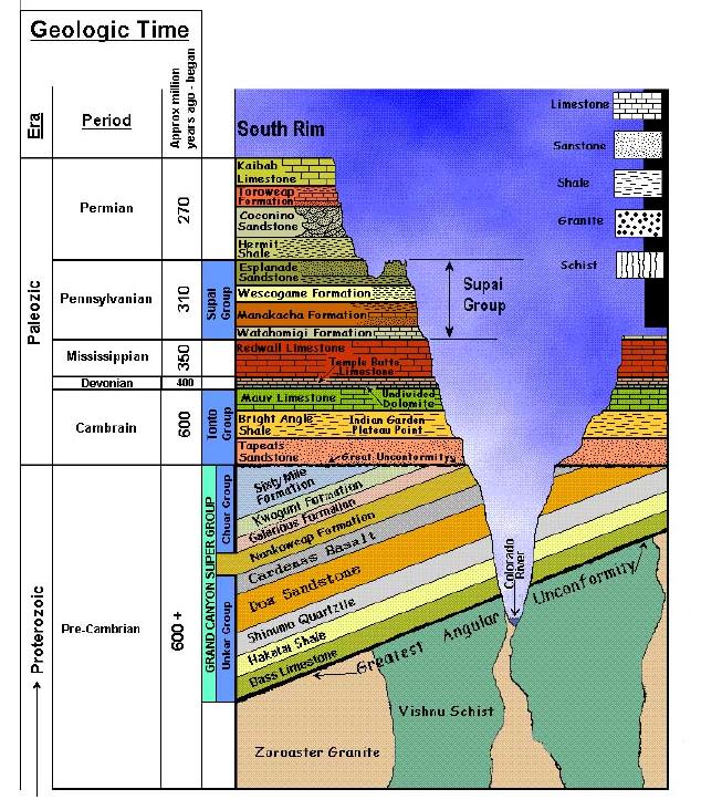